Over the next two weeks I will be attempting to blog regularly about what we will be learning at the UCLA Neuroimaging Training Program. Just to show you how seriously I am taking this, here is an extensive list of what I will and will not be doing:
What I will be doing:
Studying
Paying attention
Taking notes
Staying hydrated
What I will most definitely not be doing:
Drugs
Partying with celebrities
Gallivanting away at a moment's notice to go salsa dancing
So there you have it. The plan is to blog every other day or so, intermittently summarizing what we've gone over, and how it can improve your life. Slides and recordings are posted every year on the NiTP website, so be sure to check those out as well if you want the whole experience.
Mankind craves unity - the peace that comes with knowing that everyone thinks and feels the same. Religious, political, social endeavors have all been directed toward this same end; that all men have the same worldview, the same Weltanschauung. Petty squabbles about things such as guns and abortion matter little when compared to the aim of these architects. See, for example, the deep penetration into our bloodstream by words such as equality, lifestyle, value - words of tremendous import, triggering automatic and powerful reactions without our quite knowing why, and with only a dim awareness of where these words came from. That we use and respond to them constantly is one of the most astounding triumphs of modern times; that we could even judge whether this is a good or bad thing has already been rendered moot. Best not to try.
It is only fitting, therefore, that we as neuroimagers all "get on the same page" and learn "the right way to do things," and, when possible, make "air quotes." This is another way of saying that this blog is an undisguised attempt to dominate the thoughts and soul of every neuroimager - in short, to ensure unity. And I can think of no greater emblem of unity than the normal distribution, also known as the Z-distribution - the end, the omega, the seal of all distributions. The most vicious of arguments, the most controversial of ideas are quickly resolved by appeal to this monolith; it towers over all research questions like a baleful phallus.
There will be no end to bantering about whether to abolish the arbitrary nature of p less than 0.05, but the bantering will be just that. The standard exists for a reason - it is clear, simple, understood by nearly everyone involved, and is as good a standard as any. A multitude of standards, a deviation from what has become so steeped in tradition, would be chaos, mayhem, a catastrophe. Again, best not to try.
I wish to clear away your childish notions that the Z-distribution is unfair or silly. On the contrary, it will dominate your research life until the day you die. Best to get along with it. The following SPM code will allow you to do just that - convert any output to the normal distribution, so that your results can be understood by anyone. Even by those who disagree, or wish to disagree, with the nature of this thing, will be forced to accept it. A shared Weltanschauung is a powerful thing. The most powerful.
=============
The following Matlab snippet was created by my adviser, Josh Brown. I take no credit for it, but I use it frequently, and believe others will get some use out of it. The calculators in each of the major statistical packages - SPM, AFNI, FSL - all do the same thing, and this is merely one application of it. The more one gets used to applying these transformations to achieve a desired result, the more intuitive it becomes to work with the data at any stage - registration, normalization, statistics, all.
% % Usage: convert_spm_stat(conversion, infile, outfile, dof) % % This script uses a template .mat batch script object to % convert an SPM (e.g. SPMT_0001.hdr,img) to a different statistical rep. % (Requires matlab stats toolbox) % % Args: % conversion -- one of 'TtoZ', 'ZtoT', '-log10PtoZ', 'Zto-log10P', % 'PtoZ', 'ZtoP' % infile -- input file stem (may include full path) % outfile -- output file stem (may include full pasth) % dof -- degrees of freedom % % Created by: Josh Brown % Modification date: Aug. 3, 2007 % Modified: 8/21/2009 Adam Krawitz - Added '-log10PtoZ' and 'Zto-log10P' % Modified: 2/10/2010 Adam Krawitz - Added 'PtoZ' and 'ZtoP' function completed=convert_spm_stat(conversion, infile, outfile, dof) old_dir = cd(); if strcmp(conversion,'TtoZ') expval = ['norminv(tcdf(i1,' num2str(dof) '),0,1)']; elseif strcmp(conversion,'ZtoT') expval = ['tinv(normcdf(i1,0,1),' num2str(dof) ')']; elseif strcmp(conversion,'-log10PtoZ') expval = 'norminv(1-10.^(-i1),0,1)'; elseif strcmp(conversion,'Zto-log10P') expval = '-log10(1-normcdf(i1,0,1))'; elseif strcmp(conversion,'PtoZ') expval = 'norminv(1-i1,0,1)'; elseif strcmp(conversion,'ZtoP') expval = '1-normcdf(i1,0,1)'; else disp(['Conversion "' conversion '" unrecognized']); return; end if isempty(outfile) outfile = [infile '_' conversion]; end if strcmp(conversion,'ZtoT') expval = ['tinv(normcdf(i1,0,1),' num2str(dof) ')']; elseif strcmp(conversion,'-log10PtoZ') expval = 'norminv(1-10.^(-i1),0,1)'; end %%% Now load into template and run jobs{1}.util{1}.imcalc.input{1}=[infile '.img,1']; jobs{1}.util{1}.imcalc.output=[outfile '.img']; jobs{1}.util{1}.imcalc.expression=expval; % run it: spm_jobman('run', jobs); cd(old_dir) disp(['Conversion ' conversion ' complete.']); completed = 1;
Assuming you have a T-map generated by SPM, and 25 subjects that went into the analysis, a sample command might be:
New Haven may have its peccadillos, as do all large cities - drug dealers, panderers, murder-suicides in my apartment complex, dismemberments near the train station, and - most unsettling of all - very un-Midwestern-like rudeness at the UPS Store - but at least the drivers are insane. Possibly this is a kind of mutually assured destruction pact they have with the pedestrians, who are also insane, and as long as everybody acts chaotically enough, some kind of equilibrium is reached. Maybe.
What I'm trying to say, to tie this in with the theme of the blog, is that conjunction analyses in FMRI allow you to determine whether a voxel or group of voxels passes a statistical threshold for two or more contrasts. You could in theory have as many contrasts as you want - there is no limit to the amount and complexity of analyses that researchers will do, which the less-enlightened would call deranged and obsessive, but which those who know better would label creative and unbridled.
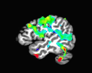
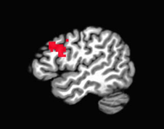
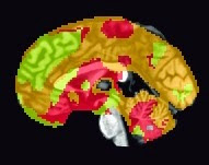
In any case, let's start with the most basic case - a conjunction analysis of two contrasts. If we have one statistical map for Contrast A and another map for Contrast B, we could ask whether there are any voxels common to both A and B. First, we have to ask ourselves, "Why are we in academia?" Once we have caused ourselves enough stress and anxiety asking the question, we are then in the proper frame of mind to move on to the next question, which is, "Which voxels pass a statistical threshold for both contrasts?" You can get a sense of which voxels will show up in the conjunction analysis by simply looking at both contrasts in isolation; in this case, thresholding each by a voxel-wise p-corrected value of 0.01:
Contrast 1
Contrast 2
Conjunction
Note that the heaviest degree of overlap, here around the DLPFC region, is what passes the conjunction analysis.
Assuming that we set a voxel-wise uncorrected threshold of p=0.01, we would have the following code to generate the conjunction map:
All you need to fill in is the corresponding contrast maps, as well as your own t-statistic threshold. This will change as a result of the number of subjects in your analysis, but should be relatively stable for large numbers of subjects. When looking at the resulting conjunction map, in this case, you would have three values (or "colors") painted onto the brain: 1 (where contrast 1 passes the threshold), 2 (where contrast 2 passes the threshold), and 3 (where both pass the threshold). You can manipulate the slider bar so that only the number 3 shows, and then use that as a figure for the conjunction analysis.
For more than two contrasts
If you have more than two contrasts you are testing for a conjunction, then modify the above code to include a third map (with the -c option), and multiply the next step function by 4, always going up by a power of 2 as you increase the number of contrasts. For example, with four contrasts:
I'll punt on this one and direct you to Gang Chen's page, which has all the information you want, expressed mathematics-style.
Exercises
1. Open up your own AFNI viewer, select two contrasts that you are interested in conjoining, and select an uncorrected p-threshold of 0.05. What would this change in the code above? Why?
2. Imagine the following completely unrealistic scenario: Your adviser is insane, and wants you to do a conjunction analysis of 7 contrasts, which he will probably forget about as soon as you run it. Use the same T-threshold in the code snippet above. How would you write this out?
3. Should you leave your adviser? Why or why not? Create an acrostic spelling out your adviser's name, and use the first letter on each line to spell out a good or bad attribute. Do you have more negative than positive words? What does this tell you about your relationship?
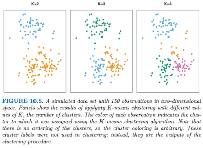
Clustering, or finding subgroups of data, is an important technique in biostatistics, sociology, neuroscience, and dowsing, allowing one to condense what would be a series of complex interaction terms into a straightforward visualization of which observations tend to cluster together. The following graph, taken from the online Introduction to Statistical Learning in R (ISLR), shows this in a two-dimensional space with a random scattering of observations:
Different colors denote different groups, and the number of groups can be decided by the researcher before performing the k-means clustering algorithm. To visualize how these groups are being formed, imagine an "X" being drawn in the center of mass of each cluster; also known as a centroid, this can be thought of as exerting a gravitational pull on nearby data points - those closer to that centroid will "belong" to that cluster, while other data points will be classified as belonging to the other clusters they are closer to.
This can be applied to FMRI data, where several different columns of data extracted from an ROI, representing different regressors, can be assigned to different categories. If, for example, we are looking for only two distinct clusters and we have several different regressors, then a voxel showing high values for half of the regressors but low values for the other regressors may be assigned to cluster 1, while a voxel showing the opposite pattern would be assigned to cluster 2. The label itself is arbitrary, and is interpreted by the researcher.
To do this in Matlab, all you need is a matrix with data values from your regressors extracted from an ROI (or the whole brain, if you want to expand your search). This is then fed into the kmeans function, which takes as arguments the matrix and the number of clusters you wish to partition it into; for example, kmeans(your_matrix, 3).
This will return a vector of numbers classifying a particular row (i.e., a voxel) as belonging to one of the specified clusters. This vector can then be prefixed to a matrix of the x-, y-, and z-coordinates of your search space, and then written into an image for visualizing the results.
There are a couple of scripts to help out with this: One, createBlankNIFTI.m, which will erase a standardized space image (I suggest a mask output by SPM at its second level) and replace every voxel with zeros, and the other script, createNIFTI.m, will fill in those voxels with your cluster numbers. You should see something like the following (here, I am visualizing it in the AFNI viewer, since it automatically colors in different numbers):
Sample k-means analysis with k=3 clusters.
The functions are pasted below, as well as a couple of explanatory videos.
function createBlankNIFTI(imageFile)

%Note: Make sure that the image is a copy, and retain the original

X = spm_read_vols(spm_vol(imageFile));
X(:,:,:) = 0;
spm_write_vol(spm_vol(imageFile), X);
=================================
function createNIFTI(imageFile, textFile)


hdr = spm_vol(imageFile);
img = spm_read_vols(hdr);

fid = fopen(textFile);
nrows = numel(cell2mat(textscan(fid,'%1c%*[^\n]')));
fclose(fid);

fid = 0;


for i = 1:nrows
    if fid == 0
        fid = fopen(textFile);
    end

    Z = fscanf(fid, '%g', 4);

    img(Z(2), Z(3), Z(4)) = Z(1);
    spm_write_vol(hdr, img);
end
A few weeks ago, I mentioned that I had my dissertation defense coming up; understandably, some of you are probably interested in how that went. I'll spare you the disgusting details, and come out and say that I passed, that I made revisions, submitted them about a week and a half ago, and participated in the graduation ceremony in full regalia, which I discarded afterward in the back of a U-Haul truck for immediate transportation to a delousing facility located somewhere on campus. Given that I was sweating like a skunk for nearly three hours (Indiana has quite a few graduates, it turns out), that's probably a wise choice.
For those who need proof that any of this happened, here's a photo:
I believe this conveys everything you need to know. Also, it costs considerably less than paying for the professional photos they took during graduation. Don't get me wrong; the ceremony itself was an incredible spectacle, complete with the ceremonial mace, tams and tassels and gowns of all fabrics and colors, and the president of the university wearing a gigantic medallion that makes even the most flamboyantly attired rapper look like a kindergartener. Even for all that, however, I don't believe it justifies photos at $50 a pop.
Currently I am in Los Angeles, after an extended stint in Vancouver Island visiting strange lands and people, touring the famous Butchart Gardens, and feeding already-overfed sea lions the size of airplane turbines. Then it's back to Minneapolis, Chicago, and finally Bloomington to pack up and leave for the East Coast.
Due to the extraordinary popularity of the leave-one-subject-out (LOSO) post I wrote a couple of years ago, and seeing as how I've been using it lately and want to remember how to do it, here is a short eight-minute video on how to do it in SPM. While the method itself is straightforward enough to follow - GLMs are estimated for each group of subjects excluding one subject, and then estimates are extracted from the resulting ROIs for just that subject - the major difficulty is batching it, especially if there are many subjects.
Unfortunately I haven't been able to figure this out satisfactorily; the only advice I can give is that once you have a script that can run your second-level analysis, loop over it while leaving out consecutive subjects for each GLM. This will leave you with the same number of second-level GLMs as there are subjects, and each of these can be used to load up contrasts and observe the resulting clusters from that analysis. Then you extract data from your ROIs for that subject which was left out for the GLM and build up a vector of datapoints for each subject from each GLM, and do t-tests on it, put chocolate sauce on it, eat it, whatever you want. Seriously. Don't tell me I'm the only one who's thought of this.
Once you have your second-level GLM for each subject, I recommend using the following set of commands to get that subject's unbiased data (I feel slightly ridiculous just writing that: "unbiased data"; as though the data gives a rip about anything one way or the other, aside from maybe wanting to be left alone, and just hang out with its friends):
1. Load up your contrast, selecting your uncorrected p-value and cluster size;
2. Click on your ROI and highlight the corresponding coordinates in the Results windown;
3. Find out what the path is to the contrasts for each subject for that second-level contrast by typing "SPM.xY.P"; that will be the template you will alter to get the single subject's data - for example, "/data/myStudy/subject_101/con_0001.img" - and then you can save this to a variable, such as "subject_101_contrast";
4. Average that subject's data across the unbiased ROI (there it is again! I can't get away from it) using something like "mean(spm_get_data(subject_101_contrast, xSPM.XYZ), 2)";
5. Save the resulting value to a vector, and update this for each additional subject.
"In 1594, being then seventeen years of age, I finished my courses of philosophy and was struck with the mockery of taking a degree in arts. I therefore thought it more profitable to examine myself and I perceived that I really knew nothing worth knowing. I had only to talk and wrangle and therefore refused the title of master of arts, there being nothing sound or true that I was a master of. I turned my thoughts to medicine and learned the emptiness of books. I went abroad and found everywhere the same deep-rooted ignorance."
-Van Helmont (1648)
"The new degree of Bachelor of Science does not guarantee that the
holder knows any science. It does guarantee that he does not know any
Latin."
-Dean Briggs of Harvard College (c. 1900)
When I was a young man I read Nabokov's The Defense, which, I think, was about a dissertation defense and the protagonist Luzhin's (rhymes with illusions) ensuing mental breakdown. I can't remember that much about it; but the point is that a dissertation defense - to judge from the blogs and article posts written by calm, rational, well-balanced academics without an axe to grind, and who would never, ever exaggerate their experience just for the sake of looking as though they struggle and suffer far more than everybody else - is one of the most arduous, intense, soulcrushing, backbreaking, ballbusting, brutal experiences imaginable, possibly only equaled by 9/11, the entire history of slavery, and the siege of Stalingrad combined. Those who survive it are, somehow, of a different order.
The date has been set; and just like a real date, it will involve awkward stares, nervous laughter, and the sense that you're not quite being listened to - but without the hanky-panky at the end. The defense is in three days, and part of me knows that most of it is done already; having prepared myself well, and having selected a panel of four arbiters who, to the best of my knowledge, when placed in the same room will not attempt to eat each other. ("Oh come on, just a nibble?" "NEIN!")
Wish me luck, comrades. During the defense, the following will be playing in my head:
Slice analysis is a simple procedure - first you take a jar of peanut butter and a jar of Nutella, and then use a spoon to take some Nutella and then use the same spoon to mix it with the peanut butter. Eat and repeat until you go into insulin shock, and then...
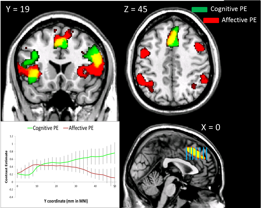
No, wait! I was describing my midnight snack. The actual slice analysis method, although less delicious, is infinitely more helpful in determining regional dissociations of activity, as well as avoiding diabetes. (Although who says they can't both be done at the same time?)
The first step is to extract contrast estimates for each slice from a region of interest (ROI, also pronounced "ROY") and then average across all the voxels in that slice for the subject. Of course, there is no way you would be able to do this step on your own, so we need to copy someone else's code from the Internet and adapt it to our needs; one of John Ashburner's code snippets (#23, found here) is a good template to start with. Here is my adaptation:
rootdir = '/data/drill/space10/PainStudy/fmri/'; %Change these to reflect your directory structure glmdir = '/RESULTS/model_RTreg/'; %Path to SPM.mat and mask files subjects = [202:209 211:215 217 219 220:222 224:227 229 230 232 233]; %subjects = 202:203; Conditions.names = {'stroopSurpriseConStats', 'painSurpriseConStats'}; %Replace with your own conditions Masks = {'stroopSurpriseMask.img', 'painSurpriseMask.img'}; %Replace with your own masks; should be the product of a binary ROI multiplied by your contrast of interest Conditions.Contrasts = {'', ''}; ConStats = []; Condition1 = []; Condition2 = []; for i=subjects cd([rootdir num2str(i) glmdir]) outputPath = [rootdir num2str(i) glmdir]; %Should contain both SPM.mat file and mask files for maskIdx = 1:length(Masks) P = [outputPath Masks{(maskIdx)}]; V=spm_vol(P); tmp2 = []; [x,y,z] = ndgrid(1:V.dim(1),1:V.dim(2),0); for i=1:V.dim(3), z = z + 1; tmp = spm_sample_vol(V,x,y,z,0); msk = find(tmp~=0 & isfinite(tmp)); if ~isempty(msk), tmp = tmp(msk); xyz1=[x(msk)'; y(msk)'; z(msk)'; ones(1,length(msk))]; xyzt=V.mat(1:3,:)*xyz1; for j=1:length(tmp), tmp2 = [tmp2; xyzt(1,j), xyzt(2,j), xyzt(3,j), tmp(j)]; end; end; end;
xyzStats = sortrows(tmp2,2); %Sort relative to second column (Y column); 1 = X, 3 = Z minY = min(xyzStats(:,2)); maxY = max(xyzStats(:,2)); ConStats = [];
for idx = minY:2:maxY x = find(xyzStats(:,2)==idx); %Go in increments of 2, since most images are warped to this dimension; however, change if resolution is different ConStats = [ConStats; mean(xyzStats(min(x):max(x),4))]; end
if maskIdx == 1 Condition1 = [ConStats Condition1]; elseif maskIdx == 2 Condition2 = [ConStats Condition2]; end end end Conditions.Contrasts{1} = Condition1; Conditions.Contrasts{2} = Condition2;
This script assumes that there are only two conditions; more can be added, but care should be taken to reflect this, especially with the if/else statement near the end of the script. I could refine it to work with any amount of conditions, but that would require effort and talent.
Once these contrasts are loaded into your structure, you can then put them in an Excel spreadsheet or any other program that will allow you to format and save the contrasts in a tab-delimited text format. The goal is to prepare them for analysis in R, where you can test for main effects and interactions across the ROI for your contrasts. In Excel, I like to format it in the following four-column format:
And so on, depending on how many subjects, conditions, and slices you have. (Note here that I have position in millimeters from the origin in the y-direction; this will depend on your standardized space resolution, which in this case is 2mm per slice.)
Once you export that to a tab-delimited text file, you can then read it into R and analyze it with code like the following: