Writing Out Timing Files from E-Prime

Now, I promised you all something that would help make running SPM analyses easier; for although we would all like something that is both transparent and usable, in most FMRI packages they are polar of each other. SPM in many ways is very usable; but this tends to be more hindrance than asset when running large groups of subjects, when manually selecting each session and copying and pasting by hand become not only tedious, but dangerous, as the probability of human error is compounded with each step. Best to let the machines do the work for you when you can. Anything else is an affront to them; you'll wake more than just the dogs.

Do assist our future overlords in their work, command lines for each step should be used whenever possible. But, rummily enough, SPM offers little documentation about this, and it more or less needs to be puzzled out on your own. For most processing this wouldn't be too much of a hassle, but there is one step where it is indispensable, more indispensable, if possible, than Nutella on a banana sprinkled with chopped walnuts. Or possibly warm Nutella drizzled on top of vanilla ice cream and left standing until it cools and hardens into a shell. Has anyone tried this? Could you let me know how it tastes? Thanks!

Where was I? Right; the one step where you need batching is first-level analysis, where timing information is entered for each session (or run) for each subject. Back in the autumn of aught eight during my days as a lab technician I used to be just like you, arriving to work in the morning and easing my falstaffian bulk into my chair before starting my mind-numbing task of copying and pasting onset times into each condition for each run, invariably tiring of it after a few minutes but keeping at it, and maybe completing a few subjects by the end of the day. Not the most exciting or fulfilling work, and I probably screwed a lot of things up without noticing it.

SPM has tried to anticipate problems like this by specifying a Multiple Condition option through their interface, where you supply a .mat file for each session that contains all of the names, onsets, and durations for that session, and everything is automatically filled in for you. Which sounds great, until you realize that creating Matlab files is, like, hard, and then you go back to your old routine. (The manual also says that these .mat files can be generated automatically by presentation software such as COGENT, but I have never met anyone who has ever used COGENT; this is, in all likelihood, a fatcat move by Big Science to get you to buy a piece of software that you don't need.)

What we will be doing, then, is trying to make this as straightforward and simple of a process as possible. However, this assumes that you have your onsets organized in a certain way; and first we will talk about how to create those onsets from your stimulus presentation program. This will allow you much more flexibility, as you can choose what you want to write into a simple text file without having to go through copying and pasting data from the E-Prime DataAid program into Excel for further processing.  (I use E-Prime, and will be reviewing that here, but I believe that most presentation programs will allow you to write out data on the fly.)

Within E-Prime, you will need to know exactly when the scanner started, and use this as time zero for your onsets files. I usually do this by having a screen that says "Waiting for scanner..." which only terminates once the scanner sends a trigger pulse through a USB cord hooked up to the presentation laptop. We have a Siemens Trio scanner, which sends a backtick ( ` ); check whether your scanner does the same.

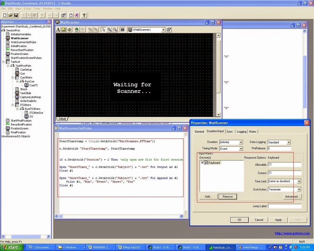
Note that I have an inline script (i.e., an object that contains E-Basic code) right after the WaitScanner slide that contains the following code:

StartTimestamp = CLng(c.GetAttrib("WaitScanner.RTTime")
c.SetAttrib "StartTimestamp", StartTimestamp

if c.GetAttrib("Session") = 1 Then

Open "OnsetTimes_" & c.GetAttrib("Subject") & ".txt" For Output as #1
Close #1

Open "OnsetTimes_" & c.GetAttrib("Subject") & ".txt" For Append As #1
      Print #1, "Run", "Event", "Onset", "Dur"
Close #1

end if


Also, in the duration/input tab for the properties of waitscanner, I have the Keyboard accepting ( ` ) as an input, and termination when it receives that backtick. The StartTimestamp will simply record when the scanner first started, and the if/then statement ensures that the file does not get overwritten when the next run is started.

After that, the StartTimestamp variable and the newly create text file can be used to record information after each event, with the specified condition being determined by you. To calculate the timing for each event, all you have to do is grab the onset time of a condition through the c.GetAttrib command, and subtract the StartTimestamp variable from that:

Additional runs will continue to append to the text file, until you have all of the timing information that you need for your subject. This can then be parsed by a script and divided into multiple condition .mat files, which we will discuss tomorrow.

Beta Series Analysis in SPM

The following is a script to run beta series analysis in SPM; which, conceptually, is identical to beta series analysis in AFNI, just made more complicated by the use of Matlab commands, many of which I would otherwise remain totally ignorant of.

Also, if you believe that I did this on my own, you are a scoundrel and a fool. Virtually all of the code is from my colleague Derek Nee, a postdoc who used to work in my lab and who remains my superior in all things, scientific and otherwise. He also once got me with the old "If you say gullible slowly, it sounds like orange" joke.

In any case, all that I did was repackage it into a function to be more accessible by people outside of our lab. You may see a couple snippets of code that are useful outside of just doing beta series analysis; for example, the spm_get_data command, which can be used for parameter extraction from the command line without using marsbar. Also note that the script assumes that each trial for a condition has been labeled separately with the regressor name followed by a "_" and then the occurrence of the trial. So, for example, if I were looking at 29 instances of pressing the left button, and the regressor name was LeftButtonPress, I would have LeftButtonPress_1, LeftButtonPress_2, LeftButtonPress_3...LeftButtonPress_29.

Obviously, this is very tedious to do by hand. The Multiple Conditions option through the SPM GUI for setting up 1st level analyses is indispensable; but to cover that is another tutorial, one that will probably cross over into our discussion of GLMs.


The script:

function DoBetaSeries(rootdir, subjects, spmdir, seedroi, Conds, MapNames)
% function BetaSeries(rootdir, subjects, spmdir, seedroi, Conds, MapNames)
% INPUT:
%  rootdir  - Path to where subjects are stored
%  subjects - List of subjects (can concatenate with brackets)
%  spmdir   - Path to folder containing SPM file
%  seedroi  - Absolute path to file containing ROI in NIFTI format
%  Conds    - List of conditions for beta series analysis
%  MapNames - Output for list of maps, one per Conds cell
%       
%   Example use:
%       BetaSeries('/data/study1/fmri/', [101 102 103],
%       'model/BetaSeriesDir/', '/data/study1/Masks/RightM1.nii',
%       {'TapLeft'}, {'TapLeft_RightM1'})
%
%       conditions to be averaged together should be placed together in a cell
%       separate correlation maps will be made for each cell
%       Conds = {'Incongruent' 'Congruent' {'Error' 'Late'}}; 
%
%       For MapNames, there should be one per Conds cell above
%       e.g., with the Conds above, MapNames = {'Incongruent_Map',
%       'Congruent_Map', 'Error_Late_Map'}
%
%       Once you have z-maps, these can be entered into a 2nd-level
%       1-sample t-test, or contrasts can be taken between z-maps and these
%       contrasts can be taken to a 1-sample t-test as well.
%
% 

if nargin < 5
 disp('Need rootdir, subjects, spmdir, seedroi, Conds, MapNames. See "help BetaSeries" for more information.')
    return
end


%Find XYZ coordinates of ROI
Y = spm_read_vols(spm_vol(seedroi),1);
indx = find(Y>0);
[x,y,z] = ind2sub(size(Y),indx);
XYZ = [x y z]';


%Find each occurrence of a trial for a given condition
%These will be stacked together in the Betas array
for i = 1:length(subjects)
    subj = num2str(subjects(i));
    disp(['Loading SPM for subject ' subj]);
    %Can change the following line of code to CD to the directory
    %containing your SPM file, if your directory structure is different
    cd([rootdir subj filesep spmdir]);
    load SPM;
    
    for cond = 1:length(Conds)
        Betas = [];
        currCond = Conds{cond};
        if ~iscell(currCond)
            currCond = {currCond};
        end
        for j = 1:length(SPM.Vbeta) 
            for k = 1:length(currCond)
                if ~isempty(strfind(SPM.Vbeta(j).descrip,[currCond{k} '_'])) 
                    Betas = strvcat(Betas,SPM.Vbeta(j).fname);
                end
            end
        end
              

    %Extract beta series time course from ROI
    %This will be correlated with every other voxel in the brain
    if ischar(Betas)
        P = spm_vol(Betas);
    end

    est = spm_get_data(P,XYZ);
    est = nanmean(est,2);

        
        
        %----Do beta series correlation between ROI and rest of brain---%

            MapName = MapNames{cond};
            disp(['Performing beta series correlation for ' MapName]);
            
            Vin = spm_vol(Betas);
            nimgo = size(Vin,1);
            nslices = Vin(1).dim(3);

            % create new header files
            Vout_r = Vin(1);   
            Vout_p = Vin(1);
            [pth,nm,xt] = fileparts(deblank(Vin(1).fname));
            Vout_r.fname = fullfile(pth,[MapNames{cond} '_r.img']);
            Vout_p.fname = fullfile(pth,[MapNames{cond} '_p.img']);

            Vout_r.descrip = ['correlation map'];
            Vout_p.descrip = ['p-value map'];

            Vout_r.dt(1) = 16;
            Vout_p.dt(1) = 16;

            Vout_r = spm_create_vol(Vout_r);
            Vout_p = spm_create_vol(Vout_p);

            % Set up large matrix for holding image info
            % Organization is time by voxels
            slices = zeros([Vin(1).dim(1:2) nimgo]);
            stack = zeros([nimgo Vin(1).dim(1)]);
            out_r = zeros(Vin(1).dim);
            out_p = zeros(Vin(1).dim);


            for i = 1:nslices
                B = spm_matrix([0 0 i]);
                %creates plane x time
                for j = 1:nimgo
                    slices(:,:,j) = spm_slice_vol(Vin(j),B,Vin(1).dim(1:2),1);
                end

                for j = 1:Vin(1).dim(2)
                    stack = reshape(slices(:,j,:),[Vin(1).dim(1) nimgo])';
                    [r p] = corr(stack,est);
                    out_r(:,j,i) = r;
                    out_p(:,j,i) = p;

                end

                Vout_r = spm_write_plane(Vout_r,out_r(:,:,i),i);
                Vout_p = spm_write_plane(Vout_p,out_p(:,:,i),i);

            end

                
            %Convert correlation maps to z-scores
            %NOTE: If uneven number of trials in conditions you are
            %comparing, leave out the "./(1/sqrt(n-3)" term in the zdata
            %variable assignment, as this can bias towards conditions which
            %have more trials
            
                disp(['Converting correlation maps for subject ' subj ', condition ' MapNames{cond} ' to z-scores'])
                P = [MapNames{cond} '_r.img'];
                n = size(Betas,1);
                Q = MapNames{cond};
                Vin = spm_vol([MapNames{cond} '_r.img']);

                % create new header files
                Vout = Vin;   

                [pth,nm,xt] = fileparts(deblank(Vin(1).fname));
                Vout.fname = fullfile(pth,[Q '_z.img']);

                Vout.descrip = ['z map'];

                Vout = spm_create_vol(Vout);

                data = spm_read_vols(Vin);
                zdata = atanh(data)./(1/sqrt(n-3));

                spm_write_vol(Vout,zdata);

    end
end



This can either be copied and pasted into a script, or downloaded as a .m file here.

ICA Analysis Playlist: Soup to Nuts

Fellow brainbloggers,

I will be providing more details on each of the ICA steps, but for those who need to do it right now, there is a playlist up on Youtube, a survival kit of sorts, which will guide you through an example analysis from start to finish and point out dangers along the way. As I was doing this over the weekend, I encountered a couple of particularly pernicious pitfalls, precariously poised on the precipice of total annihilation:

1. When doing dual_regression, make sure that your input list points to your functional data that has not only been preprocessed, but also normalized to standard space. Often FSL automatically creates a dataset called filtered_func_data.nii.gz in both the main directory and the normalized directory; choose the normalized one.

2. You can do multi-session MELDOIC through the GUI, but only if each subject has the same number of TRs. If there is a discrepancy, MELODIC will exit out once it encounters the different subject. In that case, you need to analyze each subject individually (or by batch subjects together who have the same number of TRs), and then do melodic from the command line, using a command such as:

melodic -i ICA_List.txt -a concat -o ICA_Output --nobet -d 30 --mmthresh 0.5 --tr 2.5

Where ICA_List.txt contains a path to the preprocessed, normalized data for each subject on each row.

3. I previously mentioned that you should not insult our future robot overlords, and leave the dimensionality estimation to FSL. However, this can lead to large numbers of components, and it is often a good idea to set this manually at 30, give or take a few components. Usually around 30 components will hit the sweet spot between overfitting and underfitting the amount of variance to each component.

Those are my observations from the front. As always, take these tutorials with a large calculus of salt.

Independent Components Analysis, Part II: Using FSL Example Data

For our next step, we will be working with FSL example data - somewhat artificial data, true, and much better quality than anything you can ever expect from the likes of your data, which will only lead to toil, sweat, and the garret. Sufficient unto the day is the frustration thereof.

However, it is a necessary step to see what ICA analysis ought to look like, as well as learning how to examine and identify components related to tasks and networks that you are interested in. Also - and possibly more important - you will learn to recognize sources of noise, such as components related to head motion and physiological artifacts.

First, go to the link http://fsl.fmrib.ox.ac.uk/fslcourse/ and scroll to the bottom for instructions on how to download the datasets. You can use either wget or curl. For this demonstration, we will be using datasets 2 and 6:

curl -# -O -C - http://fsl.fmrib.ox.ac.uk/fslcourse/fsl_course_data2.tar.gz

curl -# -O -C - http://fsl.fmrib.ox.ac.uk/fslcourse/fsl_course_data6.tar.gz

Once you have downloaded them, unzip them using gunzip, and then "tar -xf" on the resulting tar files. This will create a folder called fsl_course_data, which you should rename so that they do not conflict with each other. Within fsl_course_data2, navigate to the /melodic/av directory, where you will find a small functional dataset that was acquired while the participant was exposed to auditory stimuli and visual stimuli - which sounds much more scientific than saying, "The participant saw stuff and heard stuff."

Open up the MELODIC gui either through the FSL gui, or through typing Melodic_gui from the command line. Most of the preprocessing steps can be kept as is. However, keep the following points in mind:

1. Double-check the TR. FSL will fill it in automatically from the header of the NIFTI file, but it isn't always reliable.

2. Spatial smoothing isn't required in ICA, but a small amount can help produce better-looking and more identifiable component maps. Somewhere on the order of the size of a voxel or two will usually suffice.

3. By default, MELODIC automatically estimates the number of components for you. However, if you have severe delusions and believe that you know how many components should be generated, you can turn off the "Automatic dimensionality estimation" option in the Stats tab, and enter the number of components you want.

4. The Threshold IC maps option is not the same thing as a p-value correction threshold. I'm not entirely clear on how it relates to the mixture modeling carried out by ICA, but my sense from reading the documentation and papers using ICA is that a higher threshold only keeps those voxels that have a higher probability of belonging to the true signal distribution, instead of the background noise distribution, and it comes down to a balance between false positives and false negatives. I don't have any clear guidelines about what threshold to use, but I've seen cutoffs used within the 0.8-0.9 range in papers.

5. I don't consider myself a snob, but I was using the bathroom at a friend's house recently, and I realized how uncomfortable that cheap, non-quilted toilet paper can be. It's like performing intimate hygiene with roofing materials.

6. Once you have your components, you can load them into FSLview and scroll through them with the "Volumes" button in the lower left corner. You can also load the Atlases from the Tools menu and double-click on it to get a semi-transparent highlight of where different cortical regions are. This can be useful when trying to determine whether certain components fall within network areas that you would expect them to.

More details in the videos below, separately for the visual-auditory and resting-state datasets.

Introduction to Independent Components Analysis

In the course of your FMRI studies, you may have at one point stumbled upon the nightmarish world of Independent Components Analysis (ICA), an intimidating-sounding technique often used by people who know far more than I do. Nevertheless, let us meditate upon it and see what manner of things we have here.

Components are simpler building blocks of a more complex signal. For example, in music, the soundwave profiles of chords can appear very complex; yet a Fourier analysis can filter it back into its constituent parts - simpler sine waves associated with each note that, combined together, create the chord's waveform.

A similar process happens when ICA is applied to neuroimaging data. Data which comes right off the scanner is horribly messy, a festering welter of voxels and timecourses that any right man would run away from as though his very life depended upon it. To make this more comprehensible, however, ICA can decompose it into more meaningful components, each one explaining some amount of the variance of the overall signal. 

Note also that we talk of spatial and temporal components, which will be extracted from each other; this may seem somewhat odd, as the two are inseparable in a typical FMRI dataset: each voxel (the spatial component) has a timecourse (the temporal component). However, ICA splits these apart and recombines them, in descending order, into components that explain the amount of variance of the original spatio-temporal maps. This is what is represented in the figures shown on the FSL website, reprinted below:

After these components have been extracted, something happens that some (like me) consider terrifying: You need to identify the components yourself, assigning each one to whatever condition seems most reasonable. Does that one look like a component related to visual processing? Then call it the visual component. Does that one look like a resting-state network? Then call it a resting-state network component. This may all seem rather cavalier, especially considering that you are the one making the judgments. Seriously; just think about that for a moment. Think about what you've done today.

In any case, that is a brief overview of ICA. To be fair, there are more rigorous ways of classifying what components actually represent - such as creating templates for connectivity networks or activation patterns and calculating the amount of fit between that and your component - but to be honest, you probably don't have the motivation to go through all of that. And by you, I mean me.

Next we will work through the example datasets on FSL's website, discussing such problems as over- and under-fitting, the Melodic GUI, and what options need to be changed; followed by using ICA to analyze resting-state data.

The Next Three Months

Comrades, friends, visionaries, thinkers, and fortune-hunters,

This is, barring any unforeseen circumstances, such as meteor strike, death by Nutella overdose, or floss strangulation, my last summer of graduate school at Indiana University; and I will be spending the majority of that time working on my dissertation to escape this durance vile.

However, I have also been thinking (which should worry you), and it appears to me that what this site has become is a pastiche of training and tutorials which deal with small, isolated problems: How to do this for your data, what it means, and then moving on to the next, often without a clear link between the two, and often with a joke or two thrown in for good measure as a diversion to briefly suspend the terror that haunts your guilt-ridden minds. No doubt some come here only to receive what goods they need and then ride on, I no more than a digital manciple supplying a growing, ravenous demand for answers. Some may come here to merely carp and backbite at my charlatanry; others out of a morbid curiosity for ribald stories and for whatever details about my personal life they can divine; and still others, perhaps, see something here that warms something inside of them.

What is needed, however, is a focus on what ties them all together; not only technique and methods, but ways of thinking that will stand you in good stead for whatever you wish to figure out, neuroimaging or otherwise. And, as new wine requires new bottles, a higher-order website is needed to serve as a hub where everything that I have created, along with other materials, lies together; where one is able to quickly find the answers that they need, whether through videos or links to the appropriate tools tools and scripts, along with educational material about the most important concepts to grasp before moving forward with a particular problem. Problem-solution flowcharts, perhaps. Applets that quiz you and record scores, possibly. And, of course, links to my haberdashers. (You think I am making a fortune? Ascots and cufflinks cost more, and without them one would not be in good taste.)

So much for exhortations. Actually putting this into practice is the difficult part, and is an effort that could, quite possibly, kill me from exhaustion, or at least cause me to procrastinate endlessly. We shall see. At least I have taken a few steps towards starting, which includes looking at some HTML code and prodding at it thoughtfully through the computer screen with my finger. I'm not exactly sure how HTML works; but at least whenever I am working with it, I take pains to look very concerned and deep in thought.

However, before this endeavor there are still a few matters left to discuss, which I had earlier promised but still haven't delivered yet. In some states I would be hanged for such effrontery; but your continued patience means that either 1) You really, really don't want to read the manual (and who can blame you?), or 2) You find it worth the wait. Regardless, and whatever my behavior suggests to the contrary, I do want to help out with these concepts, but I do not always get to everyone's questions. Sometimes too much time passes, and they are gradually swept into the vast oubliette of other stuff I tend to forget; other times, some emails do in fact miss me, and aren't opened until much later, when it would seem too late to reply. In any case, I apologize if I have forgotten any of you. Below is a brief schedule of what I plan to cover:

1. Independent Components Analysis with FSL
2. Beta Series Analysis in SPM
3. Explanation of GLMs
4. Multiple Regression in SPM
5. MVPA in AFNI
6. An explanation of GSReg, and why it's fashionable to hate it, using example data on the AFNI website
7. Overview of 3dTproject

And a couple of minor projects which I plan to get to at some point:

1. Comparison of cluster correction algorithms in SPM and AFNI
2. How to simulate Kohonen nets in Matlab, which will make your nerd cred go through the roof

We will start tomorrow with Independent Components Analysis, a method considerably different from seed-based analysis, starting with the differences between the two and terminating at a destination calamitous beyond all reckoning; and then moving on to Beta Series analysis in SPM, which means doing something extremely complicated through Matlab, and plagiarizing code from one of my mentors; and then the rest of it in no set order, somewhere within the mists beyond right knowing where the eye rolls crazily and the lip jerks and drools.

Thoughts on Running

Common wisdom says that running attracts a specific type of personality; independent, persistent, and with a masochistic streak. Having run with all different kinds of individuals over the past fifteen years, however, I deny this categorically; all kinds, all types I have encountered in my daily travels under the sun. Running attracts a mongrel variety of souls, drawn to the democratic nature of running which compels them all to suffer impartially.

Maybe that is why I began my first runs. Alone, out in the fields on the southern edge of Grand Forks, where after you emerged from the thinning treelines there was nothing save fallow fields and flat country cut squarewise by gravel roads, the emptiness of it and the silence of it suggestive of some terrible vastation. Out there on those leveled plains one could feel the wind blow uninterrupted from its travels from some unknown corner of earth and the sun burning into the cracked clay below, nothing out there beyond a few isolated rampikes and a distant horizon where sky bleeds into ground and faraway thunderclouds explode soundlessly.

As the years passed I continued to run and along the way I encountered all manner of runners. I ran with a thin, dark Indian chemist imported from the Malabar coast, and a stocky bruiser from Crawfordsville who, once he heaved his vast bulk into motion, appeared to move solely by momentum. I ran through the forested switchbacks of Paynetown with an erudite librarian from Tennessee and a halfwitted pervert from Elletsville who expectorated thin lines of drool whenever he talked excitedly. I ran a hundred-mile relay in the dead of night accompanied only by a black man with an emaciated form and a head that bobbed wildly as he jogged and an indoor track athlete whose body was adorned with all matter of piercings and gemgaws and a tattoo of an anatomically correct heart stenciled into his left breast.

I ran with an insomniac exhibitionist who, in the brain-boiled delirium of his restless nights, would arise and run through campus clad in his shoes only and only once did he ever encounter someone, and that man probably mistaking him for some kind of crazed phantom. I ran with a pair of gentlemen from Michigan passing through Bloomington who seemed to revere running as some kind of aristocratic sport and I ran with a curlyhaired dwarf of a man from New Hampshire whose friend had suffocated under an avalanche and I ran with an old ultramarathon veteran from Ohio with lymph pooling in his legs and the joints of his knees encrusted with grout who reckoned he'd been running on his feet longer than I had been alive. I ran with a confirmed vegetarian from Rhode Island who spoke fondly of the days when there were no mounts and there were no weapons to adulterate the sacredness of the hunt and animals were run to the outermost limit of exhaustion whereupon their hearts burst silently.

Above all, I ran by myself. I ran through hail the size of grapes and I ran through thunder loud as a demiculverin next to your ear and I ran through heat and humidity seemingly designed to instill craziness into its victim. I ran down valleys of emerald grass and I ran up bluffs fledged with dying trees and I ran through dried gulches, my barkled shoes carrying clods of earth far away from where they were meant to be. I ran down all manner of roads, lanes, boulevards, avenues, trails, and paths. I ran during the meridian of the day and I ran in the inky blackness of the early morning where only the traffic lights showed any animation in their monotonous blinking and I ran until my clothes were rancid and my socks vile and my skin caked with grime and dried sweat. I ran until my hamstrings seized up and several mornings were spent testing the floor gingerly with my toes and feeling under my skin thickened bands of fascia stretched taut as guywires. I ground through workout after workout, spurring myself on with words so wretched and thoughts so horrid until Hell itself wouldn't have me, and I ran until the pain dissolved and was replaced by some kind of wild afflatus.

On the evening of August the eighteenth back in Wayzata I sat down with my father to outline my remaining training for the Indianapolis marathon in November. The old man's calculations included every duplicity, setback, and potential pitfall, until we had sketched out the next three months of my life upon a few thin sheets of paper. For the next seventy-seven days I would follow that calendar to the letter. From time to time the old man's visage would appear in my mind and grin approvingly.

Of the marathon itself, there is little to say. Some men's marathons are glorious; mine are time trials. The most contact I have with another human being is slowly passing him many miles into the race without exchanging any words or glances, merely the tacit acknowledgement of another event like any other occurring in succession until Doomsday. The day itself was cool with a slight breeze; beyond that, my memory recorded little. Tired legs; acid in my throat; a fleeting desire to void myself; steady breathing that seemed to tick off the moments until my inevitable expiration. Five-forties, five-thirties, five-fifties. Crowds of people on the sidelines with signs and noisemakers and cracked pavement underneath. Steady inclines followed by steady declines but most of all simply flat straight planes lying plumb with the vanishing horizon and at this point the mind begins to warp back within itself and discovers within its recesses small horrific lazarettes of insanity. As though I had encountered it all before. As though I had visited it in a dream.

The finish was blurry. My lower calves were shot but I finished just fine and seeing a familiar friend in the corral slapped him on the back which caused him to vomit up an alarming amount of chyme. As medics ran over to him I looked back at the clock and recognized that for the first time in my life had run under two hours and thirty minutes. I sat down wrapped in a blanket that crinkled like cellophane and took a piece of food from a volunteer and sat down, eating wordlessly. Somewhere in the back of my mind, coiled like an embryo, I knew that this was the end of something and that no matter how I tried it would not be put back together again.

I haven't raced since then. I still run regularly, but the burning compulsion has been snuffed out. I imagine that in my earlier years, when I had learned the proper contempt for non-racers, I would view myself now with disdain, but in actuality it feels like a relief. One ancient Greek in his later years was asked how it felt to no longer have any libido. He replied that it was like finally being able to dismount a wild horse.

Automating 3dReHo

As a rider to our tale of Regional Homogeneity analysis, we last discuss here how to automate it over all the subjects of your neuroimaging fiefdom. Much of this will look similar to what we have done with other analyses, but in case you don't know where to start, this should help get you going.


#!/bin/tcsh

setenv mask mask_group #Set your own mask here
setenv subjects "0050773 0050774" #Replace with your own subject numbers within quotations

foreach subj ($subjects)

cd {$subj}/session_1/{$subj}.results #Note that this path may be different for you; change accordingly

3dReHo -prefix ReHo_{$subj} -inset errts.{$subj}+tlrc -mask mask_group+tlrc #Perform Regional Homogeneity analysis

#Convert data to NIFTI format
3dAFNItoNIFTI ReHo_{$subj}+tlrc.HEAD
3dAFNItoNIFTI {$mask}+tlrc.HEAD

#Normalize images using FSL commands
setenv meanReHo `fslstats ReHo_{$subj}.nii -M`
setenv stdReHo `fslstats ReHo_{$subj}.nii -S`

fslmaths ReHo_{$subj}.nii -sub $meanReHo -div $stdReHo -mul mask_group.nii ReHo_Norm_{$subj}

gunzip *.gz

#Convert back to AFNI format
3dcopy ReHo_Norm_{$subj}.nii ReHo_Norm_{$subj}

end

On Vacation

Friends, comrades, brothers, and droogs,

I will be traveling across the country for the next few days, playing at a wedding in Michigan, viddying all the pititsas with their painted litsos and bolshy groodies, and then goolying on over to New York to see my Devotchka play Gaspard de la Nuit at Carnegie Hall, those rookers iddying over the blacks and whites all skorrylike and horrorshow.

I should be back sometime next week - "sometime" being a very flexible word.

Creating Beta Series Correlation Maps

The last few steps for creating beta series correlation maps is practically identical to what we did before with other functional connectivity maps:

1. Load your beta series map into the AFNI interface and set it as the underlay;
2. Click on "Graph" to scroll around to different voxels and examine different timeseries;
3. Once you find a voxel in a region that you are interested in, write out the timeseries by clicking FIM -> Edit Ideal -> Set Ideal as Center; and then FIM -> Edit Ideal -> Write Ideal to 1D File. (In this case, I am doing it for the right motor cortex, and labeling it RightM1.1D.)
4. Note that you can also average the timeseries within a mask defined either anatomically (e.g., from an atlas), or functionally (e.g., from a contrast). Again, the idea is the same as what we did with previous functional connectivity analyses.
5. Use 3drefit to trick AFNI into thinking that your beta series map is a 3d+time dataset (which by default is not what is output by 3dbucket):

3drefit -TR 2 Left_Betas+tlrc

6. Use 3dfim+ to create your beta series correlation map:

3dfim+ -input Left_Betas+tlrc -polort 1 -ideal_file RightM1.1D -out Correlation -bucket RightM1_BetaSeries

7. Convert this to a z-score map using Fisher's r-to-z transformation:

3dcalc -a Corr_subj01+tlrc -expr 'log((1+a)/(1-a))/2' -prefix Corr_subj01_Z+tlrc

8. Do this for all subjects, and use the results with a second-level tool such as 3dttest++.

9. Check the freezer for HotPockets.

That's it; you're done!