Combining ROIs

Once you've used a tool like fslmaths, 3dcalc, or Marsbar to create a single ROI, you can combine several of these ROIs using the same tools. This might be useful, for example, when creating a larger-scale masks encompassing several different areas.

In each case, combining ROIs is simply a matter of creating new images using a calculator-like tool; think of your TI-83 from the good old days, minus those frustrating yet addictive games such as FallDown. (Personal record: 1083.) With fslmaths, use the -add flag to concatenate several different ROIs together, e.g.:

fslmaths roi1 -add roi2 -add roi3 outputfile

With AFNI:

3dcalc -a roi1 -b roi2 -c roi3 -expr '(a+b+c)' -prefix outputfile

With Marsbar is a bit more involved, but also easier since you can do it from the GUI, as shown in the following video.




Many thanks to alert reader Anonymous, who is both too cool to register a username and once scored a 1362 on FallDown. Now all you gotta do is lay back and wait for the babe stampede!

Why Do Rednecks Do It Doggy Style?

So they can both watch NASCAR.

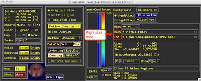
Now that I have your attention, I would like to turn to a more serious topic: Sub-brik selection in AFNI. If you have a small screen or simply too many sub-briks in your statistical dataset, it can be difficult, if not impossible, to select an appropriate sub-brik through the drop-down menu in the GUI. Instead, by right-clicking on the "OLay" or "Thr" text, you will get a scroll menu to select the sub-brik.

This, I hope, will save you countless hours of frustration and despair, and awaken your senses to the beauties of the world and touch your soul to the quick. At least, that's what I try telling myself every night when I hear the neighbors switch on NASCAR and start to get randy. Thin walls, guys!


As if a picture weren't enough, here's a video to go along with it. Since I can't help but overdo everything.

Parameter Extraction in AFNI: 3dmaskave and 3dmaskdump

Previously we showed how to extract parameters using Marsbar in SPM and featquery in FSL, and the concept is identical for AFNI. Once you have created a mask (e.g., using 3dUndump or 3dcalc), you can then extract parameter estimates from that ROI either using the tool 3dmaskave or 3dmaskdump.
3dmaskave is quicker and more efficient, and is probably what you will need most of the time. Simply supply a mask and the dataset you wish to extract from, and it will generate a single number of the average parameter estimate across all the voxels within that ROI. For example, let's say that I want to extract beta weights from an ROI centered on the left nucleus accumbens, and I have already created a 5mm sphere around that structure stored in a dataset called LeftNaccMask+tlrc. Furthermore, let's say that the beta weights I want to extract are in a beta map contained in the second sub-brik of my statistical output dataset. (Remember that in AFNI, sub-briks start at 0, so the "second" sub-brik would be sub-brik #1.) To do this, use a command like the following:

3dmaskave -mask LeftNaccMask+tlrc stats.202+tlrc'[1]'

This will generate a single number, which is the average beta value across all the voxels in your ROI.

The second approach is to use 3dmaskdump, which provides more information than 3dmaskave. This command will generate a text file that contains a single beta value at each voxel within the ROI. A couple of useful options are -noijk, to suppress the output of voxel coordinates in native space, and -xyz, to output voxel coordinates in the orientation of the master dataset (usually in RAI orientation). For example, to output a list of beta values into a text file called LeftNaccDumpMask.txt,

3dmaskdump -o LeftNaccDumpMask.txt -noijk -xyz -mask LeftNaccMask+tlrc stats.202+tlrc'[1]'

This will produce a text file that contains four columns: The first three columns are the x-, y-, and z-coordinates, and the fourth column is the beta value at that triplet of coordinates. You can take the average of this column by exporting the text file to a spreadsheet like Excel, or use a command like awk from the command line, e.g.

awk '{sum += $4} END {print "Average = ", sum/NR}' LeftNaccDumpMask.txt


Keep in mind that this is only for a single subject; when you perform a second-level analysis, usually what you will want to do is loop this over all of the subjects in your experiment, and perform a statistical test (e.g., t-test) on the resulting beta values.






Concluding Unscientific Postscript

I recently came across this recording of Schubert's Wanderer Fantasie, and I can't help but share it here; this guy's execution is damn near flawless, and, given both the time of the recording and some of the inevitable mistakes that come up, I have good reason to believe it was done in a single take. It's no secret that I do not listen to that much modern music, but it isn't that modern music is bad, necessarily; it's just that classical music is so good. Check out the melodic line around 16:30 to hear what I'm talking about.

Creating Spherical ROIs in AFNI Using 3dUndump

Regions of interest; everybody wants them, but nobody knows how to get them. However, as Megatron once said, power flows to the one who knows how; desire alone is not enough.

Aware of this, I have created a script which will disenthrall you from the pit of ignorance and give you the power to create ROIs just about anywhere you please. The script uses AFNI's 3dUndump, which creates a spherical ROI of a given radius from which parameter values can be extracted using a tool like 3dmaskdump. The rationale is similar to creating ROIs using fslmaths or SPM's marsbar; and if you understand those, using 3dUndump is essentially the same thing.

The only caveat is that you must know the orientation of your dataset before using 3dUndump. AFNI defaults to RAI orientation, in which numbers increase from right to left, anterior to posterior, and inferior to superior; in other words, coordinates to the right of the origin will be negative (since numbers decrease going from left to right), and coordinates anterior to the origin will be negative (since numbers again decrease going from posterior to anterior). Always make sure to check the orientation using a command like 3dinfo -orient before creating your ROI, or open up your anatomical dataset in the AFNI viewer and navigate to the location that you want (e.g., right nucleus accumbens) and then write down the coordinates displayed in the upper left corner of the viewer. You can also use the option -orient LPI, if you're using coordinates from a paper.

This Python script that will let you input the coordinates, and then output a dataset ROI that can be overlaid on your anatomical image. The script can be found here.


Tutorial on 3dUndump:

Tutorial on MakeSpheres.py

Capital City Half Marathon

I and my sidekick (you haven't met her) always strive to bring you the hottest, moistest tutorial videos and neuroscience-related news, but I will be traveling to Columbus, Ohio to run the Capital City half marathon this weekend. Just thought you would like to know that I run more than you do, and am faster than you will ever be in your entire life. I also don't have a TV. Did you know that? Think about that the next time you're watching TV. I'm serious.

What Good is Neuroimaging?

If there is one absolute in this universe, it is that people want more stuff. Given the choice between stuff and nothing, people will choose stuff, nine times out of ten. Therefore, as science is a business as well as an intellectual pursuit, any scientist would be well-advised to take a step back once in a while and consider whether his work makes the public feel as though that they are getting more stuff. This gets back to the divide between basic research and translational research: basic research being done more for its own sake, and to just figure stuff out; and translational research, which attempts to bridge basic scientific findings and transform them into improved technologies or therapies.

A recent article in the Journal of Cognitive Neuroscience (Moran & Zaki, 2013) addresses these very issues, stating that neuroimaging has reached a critical mass of exploratory findings through brain mapping, but in order to advance will have to take a more theoretically rigorous approach. In the good old days, it was interesting to do basic exploratory analyses to examine the functional role of large chunks of cortical real estate, such as the visual cortex, auditory cortex, and some subcortical structures. However, the authors maintain that most new exploratory brain analyses - i.e., those that simply want to find out what brain region is responsive to a certain task or a certain stimulus - are rapidly entering the far end of diminishing returns. What is needed, rather, is experiments that can adjudicate between competing theories of brain function, using forward inference to distinguish between alternative hypotheses, instead of reverse inference, which reasons that because a particular region shows more activity than normal, then a particular process must be involved (cf. Poldrack, 2006).

However, even with reverse inference, some assumptions can be made about a cognitive state. For example, with large-scale databases such as Neurosynth, one can quickly see how many studies claim that a given region is involved in a particular cognitive process. This lends more credibility to reverse inference claims that dovetail with evidence from the majority of studies, as opposed to selecting a single study that claimed to have found evidence of a cognitive process associated with a certain area, as this may be more susceptible to a false positive.

For practical uses, however, neuroimaging - and FMRI in particular - has been able to make predictions about behavior based on brain activity. For example, in a growing body of decision-making research, increased activity in the anterior insula predicted better choices in a risky decision-making task (Krawitz et al, 2010), and within a group of smokers shown anti-tobacco ads, dorso-medial prefrontal cortex activity predicted levels of a nicotine metabolite at a later follow-up (Wang et al, 2013). This seems to be a profitable avenue of neuroimaging research, as neural activity can provide more information about effective treatment programs, from drug PSAs to psychological therapies, above and beyond behavioral measures.

In light of all this, the evidence suggests that, although brain mapping for its own sake will continue to be popular, the higher-impact work appears to be shifting more emphatically in the direction of translational research. The human desire for stuff will always trump the human desire of curiosity, and the researcher would be wise to pay heed to this, lest he be swallowed up in darkness.

SPM Tutorial: Creating Contrast Images

Those of you who have ever entered a string of ones and negative-ones in SPM's contrast manager were creating contrast images (simultaneously converted into T-maps or F-maps), whether you knew it or not. It can be difficult to see exactly what is going on, but as part of creating a statistical map, SPM calls upon its mathematical tool, spm_imcalc_ui (or just spm_imcalc; but I find spm_imcalc_ui easier to understand and to use, and therefore I will focus on it).

While using the contrast manager is useful for creating relatively simple single-subject maps, you may want to then create images from those simpler images; for example, let's say you have created functional connectivity maps, but want to take the difference between two of those maps and feed the resulting contrast map into a second-level analysis. spm_imcalc_ui allows you to do this easily, and can be scripted, saving you precious time to do more important things, like take pictures of that cucumber salad sandwich or whatever you're eating and load it onto Twitter.

spm_imcalc_ui requires at least three inputs:

1. A matrix of input filenames;
2. An output file;
3. A mathematical operation to perform on the input images.

As a simple example, let's say we use the contrast manager to create two contrast images, con_0001.img and con_0002.img. Let's then say that we want to take the difference of these image to use in a second-level analysis. First, it is usually easier to assign a variable name to each file:

P1 = 'con_0001.img'; P2 = 'con_0002.img'

And then input these into spm_imcalc_ui:

spm_imalc_ui([P1; P2], 'outputImage.img', 'i1-i2'

Note that the third argument, i1-i2, calls upon reserved SPM keywords, i.e., "i1" and "i2". i1 refers to the first input image, i2 refers to the second input image, and so on.

That's really all there is to it; and from this example you can simply add more images, and perform more complex operations if you like (e.g., make one an exponent of the other, i1.^i2). Furthermore, when you have several runs, using the contrast manager can quickly become unwieldy; you can use the contrast manager to first create an image for a single regressor by positively weighting only those betas in each run corresponding to your regressor, and then when these images are created, use spm_imcalc_ui to make your contrast images. As stated previously, this allows for more flexibility in scripting from the command line, potentially saving you thousands of man-hours in cucumber-sandwich-photo-taking endeavors.

FSL Tutorial: Creating ROIs from Coordinates

Previously we covered how to create regions of interest (ROIs) using both functional contrasts and anatomical landmarks; however, FSL can also create spheres around voxel coordinates, similar to AFNI's 3dcalc or SPM's marsbar.

1. Step one is to find the corresponding voxel coordinates for your MNI coordinates, which may be based on peak voxel activation from another study, for example; to do this, open up FSLview, type in your MNI coordinates, and write down the corresponding voxel coordinates (these are shown in the bottom-left corner of FSLview). 
2. After you have written down your voxel coordinates, create a point at those coordinates using the fslmaths command. This command requires the template space that you warped to, as well as the actual x-, y-, and z-coordinates corresponding to the MNI coordinates. Give the output file a name, and make sure that the output data type ('odt') is set to float. (Example command: fslmaths avg152T1.nii.gz -mul 0 -add 1 -roi 45 1 74 1 51 1 0 1 ACCpoint -odt float)
3. Using fslmaths again, input the file containing the point created in the previous step, and specify a sphere of radius N (in millimeters) to expand around that point. Use the -fmean command, for reasons that are to remain mysterious, and provide a label for your output data set. (Example command: fslmaths ACCpoint -kernel sphere 5 -fmean ACCsphere -odt float)
4. Update on 5/18/2016: To make it a binary mask, execute one more command: fslmaths ACCsphere.nii.gz -bin ACCsphere_bin.nii.gz. The previous step creates a sphere, but with small intensities; this can be problematic if you do a featquery analysis that allows weighting of the image.

Once that is all done, use fslview to open up a template in your normalized space, and overlay your newly created sphere; double-check to make sure that it is in roughly the location where you think it should be. Now you can extract data such as parameter estimates from this ROI, using techniques similar to those covered in previous tutorials about ROIs.

Thanks to alert viewer danieldickstein, which, due to its juvenile reference to the male member, cannot possibly be his real name. Grow up, Daniel.

Abstraction and Integration in Lateral Prefrontal Cortex

Recently the journal Cerebral Cortex accepted one of our lab's papers for publication, which has made me ecstatically, deliriously happy. This represents one of the highwater marks of my publishing career, even greater than the erotically-tinged agitprop novel I published serially in my college's Pravda-inspired newspaper. Entitled A Long Caress: Twilight of the Capitalist Idols, the book followed the lives of two dreamy radicals pursued by the CIA, of which I provide an excerpt:

Boris laid aside his Chernyshevsky pamphlet and looked at Olga. Hearing his declaiming against the capitalist dogs had brought her to a fever heat; and now, as he watched her, he noticed the graceful curves of her neck, brought into relief by the delicate strands of jet-black hair gently brushing against her collarbone and the edges of her heaving bosom. She gazed at him adoringly, sloe-eyed, her cheeks flushed, the glistening sweat making her Party-issued uniform cling to her skin like fuzz on a peach. Around her waist he wrapped his strong, powerful arms, and she offered herself up like a prize.

A few miles away in an underground bunker, all of this was transmitted through a hidden wire to CIA agent John Davies. Pressing his headphones closer to his ears, Davies frowned. "Blimey," he said.

While our new paper does not come close to the rhapsodic heights of A Long Caress, it still goes a long way to resolving fundamental issues with studying different forms of abstraction. One form of abstraction, temporal abstraction, refers to maintaining information over time, with more remote events requiring correspondingly greater levels of temporal abstraction; while a related form of abstraction, relational abstraction, refers to processing higher-level information, such as complex features of stimuli. Unhappily, they are often confounded in the same experiment. This study attempted to tease apart both of these forms of abstraction, as well as independently assess the effects of integration, wherein several different pieces of information need to be collectively processed in order to make a correct response. Temporal abstraction was nonexistent, while relational abstraction effects were found in lateral premotor cortex and rostrolateral prefrontal cortex. Integration was associated with increased activation in superior frontal sulcus and frontopolar cortex, consistent with this region's handling more abstract representations between items.

A link to the paper can be found here. Documentary footage of Stalin ordering the deaths of his generals and field marshals can be found in the following video.

The Noose Tightens: Scientific Standards Being Raised

For those of you hoping to fly under the radar of reviewers and get your questionable studies published, I suggest that you do so with a quickness. A new editorial in Nature Neuroscience outlines the journal's updated criteria for methods reporting, which removes the limit on the methods section of papers, mandates reporting the data used to create figures, and requires statements on randomization and blinding. In addition, the editorial board takes a swipe at the current level of statistical proficiency in biology, asserting that

Too many biologists [and neuroscientists] still do not receive adequate training in statistics and other quantitative aspects of their subject. Mentoring of young scientists on matters of rigor and transparency is inconsistent at best. In academia, the ever-increasing pressures to publish and obtain the next level of funding provide little incentive to pursue and publish studies that contradict or confirm previously published results. Those who would put effort into documenting the validity or irreproducibility of a published piece of work have little prospect of seeing their efforts valued by journals and funders; meanwhile, funding and efforts are wasted on false assumptions.

What the editors are trying to say, I think, is that a significant number of academics, and particularly graduate students, are most lazy, benighted, pernicious race of little odious vermin that nature ever suffered to crawl upon the surface of the earth; to which I might add: This is quite true, but although we may be shiftless, entitled, disgusting vermin, it is more accurate to say that we are shiftless, entitled, disgusting vermin who simply do not know where to start. While many of us learn the basics of statistics sometime during college, much is not retained, and remedial graduate courses do little to prepare one for understanding the details and nuances of experimental design that can influence the choice of statistics that one uses. One may argue that the onus is on the individual to teach himself what he needs to know in order to understand the papers that he reads, and to become informed enough to design and write up a study at the level of the journal for which he aims; however, this implies an unrealistic expectation of self-reliance and tenacity for today's average graduate student. Clearly, blame must be assigned: The statisticians have failed us.

Another disturbing trend in the literature is a recent rash of papers encouraging studies to include more subjects, to aid both statistical reliability and experimental reproducibility. Two articles in the last issue of Neuroimage - One by Michael Ingre, one by Lindquist et al - as well as a recent Nature Neuroscience article by Button et al, take Karl Friston's 2012 Ten Ironic Rules article out to the woodshed, claiming that small sample sizes are more susceptible to false positives, and that instead larger samples should be recruited and effect sizes reported. More to the point, the underpowered studies that are published tend to be biased to only finding effects that are inordinately large, as null effects simply go unreported.

All of this is quite unnerving to the small-sample researcher, and I advise him to crank out as many of his underpowered studies as he can before larger sample sizes become the new normal, and one of the checklist criteria for any high-impact journal. For any new experiments, of course, recruit large sample sizes, and when reviewing, punish those who use smaller sample sizes, using the reasons outlined above; for then you will have still published your earlier results, but manage to remain on the right side of history. To some, this may smack of Tartufferie; I merely advise you to act in your best interests.