Surface Rendering in SPM

Because everybody loves a good surface rendering, SPM has a built-in, quick-and-dirty tool for splashing those results on your brain surface like splashing pool water at your friends while on your spring break trip to Cancun. (Swing and a miss - but hey, at least I went for it.) I think this technique is a little dated, and personally I think Freesurfer and SUMA do a much better job; but if you just want a quick figure, and if you want to at least earn the bare minimum of respect from your fellow researchers - classified as one step above slime and two steps below the macaque monkey - then this will help you earn that respect. I know what you're thinking: What about telling your fellow researchers that you dress yourself in the morning? Surprisingly, that doesn't work nearly as well.

More details on the strengths, limitations, and spraypaint-like features of surface rendering can be found in the following video.


Head Motion and Functional Connectivity

Yesterday as I was listening to a talk about diffusion tensor imaging, a professor asked about the influences of head motion on DTI data, and whether it could lead to spurious effects. Another professor vigorously denied it, stating that it was much more of a problem for bread and butter FMRI analyses, and in particular resting state functional connectivity analyses. At one point he became so animated that his monocle fell off, his collar stud came undone, and eventually he had to be physically restrained by the people sitting next to him. It was then that I knew that I should pay heed, for it is unlikely that a scientist becomes highly excited and talkative over matters that are trivial; in short, I could sense that he was talking about something important.

I have done few functional connectivity analyses in my brief life, but what I understand about them is this: You take the timecourse of one voxel - or the average timecourse over a group of voxels, also known as a "seed" - and then compare that timecourse with the timecourse of every other voxel in the brain. (When I speak of timecourses, I mean the sampled signal over time.) If it is a good fit - in other words, if there is a significantly high correlation between the timecourses - then we say that the two regions are functionally connected. This is a bit of a misnomer, as we cannot make any direct inferences about any "real" connectivity from two correlated timecourses; but it can serve as a good starting point for more sophisticated analyses, such as psychophysiological interactions (PPI; also known as context-dependent correlations) which measure changes in functional connectivity as a function of task context. For example: Does the timecourse correlation between cognitive control regions and reward-related areas change depending on whether the subject is instructed to upregulate or downregulate their gut reactions to rewarding stimuli?

One of the most popular variations of functional connectivity is something called resting state functional connectivity (rsFC), where a subject is simply instructed to relax and listen to Barry Manilow* while undergoing scanning. Functional connectivity maps are then calculated, and usually a comparison is made between a control group and an experimental or patient group, such as schizophrenics. For us FMRI researchers, this is about as close as we can get to simulating a person's natural environment where they would be relaxing and thinking about nothing in particular; except that they're in an extremely tight-fitting, noisy tube, and unable to move in any direction more than a few millimeters. Other than that, though, it's pretty normal.

These types of experiments have become all the rage in recent years, with several studies claiming to have found meaningful resting-state differences between healthy controls and several different patients populations such as schizophrenics, depressives, Nickelback fans, and drug addicts. However, a few publications have called into question some of these results, stating that many of these differences could be due to head motion. As we've talked about before, head motion can be a particularly insidious confound in any experiment, but it is especially troublesome for functional connectivity analyses. This can arise due to systematic differences between control and patient populations that are possibly confounded with motion. Take, for example, an experiment contrasting young versus older populations. Older populations are known to move more, and any observed differences in functional connectivity may be due solely to this increased motion, not underlying neural hemodynamics.

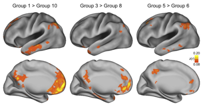
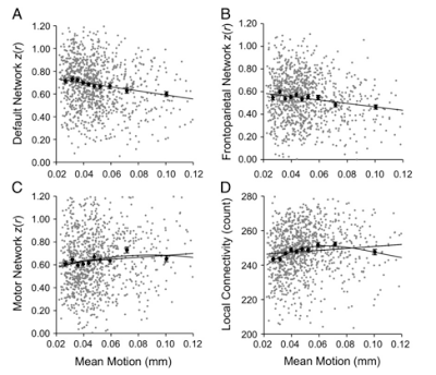
A study by Van Dijk, Sabuncu, & Bruckner (2012) looked at this in detail by scanning over a thousand (!) subjects, and binning them into ten groups based on increasing amounts of motion (e.g., group 1 had the least amount of motion, while group 10 had the most motion). The authors found decreased functional connectivity in the "default network" of the brain - usually referring to the functional connectivity between the medial prefrontal cortex and retrosplenial cingulate cortex -, decreased connectivity in the frontal-parietal network, and slightly increased local connectivity among clustered voxels, simply based on motion alone. (Keep in mind that each bin of subjects were matched as closely as possible on all other demographic measures.) Furthermore, even when comparing bins of subjects closely matched for motion (e.g., bins 5 and 6), small but significant differences in functional connectivity were seen.

Figure 3 from Van Dijk et al (2012). Functional connectivity among different networks measured as a function of head motion. Both linear and nonlinear (quadratic) terms were modeled to fit the data.

Figure 4 from Van Dijk et al (2012). Note the comparison on the far right between groups 5 and 6; the mean motion difference between these two groups is a few thousandths of a millimeter, but noticeable functional connectivity differences are still seen between the two groups.

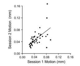
Lastly, a subset of subjects were rescanned in order to see whether motion was reliable; in other words, if a subject that moved a large amount on one day had the same tendency to move a large amount on the next day. A clear correlation was found between scanning subjects, suggesting that motion might need to be treated as a trait or individual difference, just like any other.

Figure 5 from Van Dijk et al (2012). There is a robust correlation between the movement of scanning sessions, even with the outliers removed (marked in diamonds).

So, what to do? A few recommendations are to match subjects for motion, correct motion prospectively (Ward et al, 2000), and regress out motion when performing a group-level analysis, as you would any other covariate. Apparently traditional methods of motion correction on a subject-by-subject basis are not enough, and increasing awareness of the pitfalls of between-subject motion is important for evaluating current functional connectivity analyses, and for conducting your own experiments.

This study hit me in the face like a wet mackerel since I am beginning to investigate a recent AFNI tool, 3dReHo, to do local functional connectivity analyses for publicly available datasets on the ABIDE website. However, as far as I can tell, motion limits were not used as exclusionary criteria, which may be a possible confound when examining, say, autistic children to controls. More to come soon. Or not.


*I Don't Want to Walk Without You

Learning the Fundamentals of R, Made Fun

For those of you new to R, or just curious, there is a fantastic interactive online resource for learning the fundamentals; and even those who have used R for a while may find it useful for refreshing and revitalizing their knowledge. The interface is slick (I use that word deliberately), offering incentives for completing each stage of a particular R concept or command by tracking your progress and showing how far you have come and how much farther you have to go. Finally, at the end of the day you can earn badges showing that you have successfully mastered, say, matrices and data frames, which roughly translates into getting laid anytime you want.

As some of you may know, I tried do something similar; but after a few abortive attempts at creating tutorial videos, I have decided to leave this to the experts. "Then why didn't you leave singing to the experts, instead of making a giant ass of yourself at karaoke night and picking a song by Four Non-Blondes?" Champions dare to fail.


Recital Pics

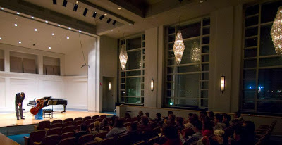
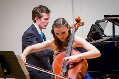
Here are a few pictures that were taken from the recital on Monday:


Taking a bow. We spent a few weeks choreographing this.


Starting things off; Mendelssohn, I think.


The rest of these are from the Grieg. Note that there is no page turner, even though my score runs for forty-five pages; by the end of the night my page-turning muscles would be bathed in lactic acid.

I know what you're thinking: What was the greater risk in your life; Playing without a page-turner, or taking a leak in the locker room shower your senior year? Difficult to say, my friends. Difficult to say.


What is Percent Signal Change? And Why are People Afraid of It?

A few years ago when I was writing up my first publication, I was gently reprimanded by a postdoc for creating a figure showing my results in percent signal change. After boxing my ears and cuffing me across the pate, he exhorted me to never do that again; his tone was much the same as parents telling their wayward daughters, recently dishonored, to never again darken their door.

Years later, I am beginning to understand the reason for his outburst; much of the time what we speak of as percent signal change, really isn't. All of the major neuroimaging analysis packages scale the data to compare signal across sessions and subjects, but expressing it in terms of percent signal change can be at best misleading, at worst fatal.

Why, then, was I compelled to change my figure to parameter estimates? Because what we usually report are the beta weights themselves, which are not synonymous with percent signal change. When we estimate a beta weight, we are looking at the amount of scaling to best match a canonical BOLD response to the raw data; a better approximation of true percent signal change would be the fitted response, and not the beta weight itself.


Even then, percent signal change is not always appropriate: recall the term "global scaling." This means comparing signal at each voxel against a baseline average of signal taken from the entire brain; this does not take into consideration intrinsic signal differences between, say, white and grey matter, or other tissue classes that one may encounter in the wilderness of those few cubic centimeters within your skull.

You can calculate more accurate percent signal change; see Gläscher (2009), or the MarsBar documentation.

Not everybody should analyze FMRI data; but if they cannot contain, it is better for one to be like me, and report parameter estimates, than to report spurious percent signal change, and burn.

Hot, Hot, HOT: Blog Dedicated to MVPA


In my whole world-wide wandering, I have concluded that nobody really knows what multivoxel pattern analysis (MVPA) is. For example, a couple of days ago I asked the checkout cashier at Target what MVPA was; he looked at me like some loutish knight beriddled by a troll.

I had nearly given up trying to understand what it was, until I stumbled upon this blog dedicated to vivisecting MVPA so that you can peer into the inner workings of this gruesome monstrosity. After having read this blog for the better part of an afternoon, I have concluded that it is able to make your wildest dreams come true and can answer any questions you could possibly have about MVPA, including discussions on the effect of different experiment parameters on classification accuracy, what a searchlight algorithm is, and what MVPA detects, exactly. It also includes, as far as I can tell, the only convincing argument in favor of allowing people to keep midgets as pets.

The author is a far more dedicated instructor than I am, with large swaths of R code accompanying most of the tutorials so that you can get a better feel for what's going on. I give this baby a 10/10.

Cello Recital: Mendelssohn, Bach, & Grieg

For any of those reading this who live in the Bloomington area, tomorrow I will be accompanying for a cello recital which includes, among other pieces, the Grieg cello sonata in A Minor, Op. 36. This one is a beast, and by far the largest and most demanding cello piece I have yet accompanied (although the Strauss and Mendelssohn cello sonatas are close contenders); but it's also epic in scope, features both displays of dazzling virtuosity and moments of heartstopping intimacy, and has a finale guaranteed to bring down the house. In short, it has all of the qualities I idolize about classical music; which, I hope, will awaken some powerful longing for the beautiful and the sublime within even the most naive listener.


Time: 7:00pm, Monday, February 25th
Location: Ford Hall (2nd Floor of the Simon Music Center, near the corner of 3rd & Jordan)

====Program====

Mendelssohn: Lied Ohne Worte, Op. 109

Bach: Cello Suite #4 in E-Flat Major, BMV 1010

Grieg: Cello Sonata in A Minor, Op. 36
   I. Allegro Agitato - Presto - Prestissimo
   II. Andante Molto Tranquilo
   III. Allegro Molto e Marcato


Using SPM.mat to Stay on Track (II)

Previously I discoursed at length upon the fatalistic nature of FMRI analysis, and how it leads to disorientation, depression, anxiety, and, finally, insanity. Those who are engaged in such a hopeless enterprise are easily identified by the voids that swirl like endless whorls within their eyes. I once knew a man driven out of his wits by just such an interminable cycle; he was found five days later on the sandy deserts of southern Indiana, ragged and filthy and babbling in alien tongues, scraping with pottery shards the boils that stippled his skin as though they had been painted on. Curse SPM, and die.

For those willing to prolong their agony, however, it is useful to know exactly what is contained within the SPM structure. Although not well-documented (if at all) on the SPM website, there are vast riches of information you can assay within the depths of the scripts themselves, which can be found in your spm8/spm5 library. (If they are in your path, you should be able to open them from anywhere; e.g., using a command such as "open spm_getSPM".) I have copied and pasted below the information from three such scripts, as well as a brief description about what they do. Good fortune to you.


================================================


1) spm_getSPM: Provides information about the xSPM structure which is updated each time Results are loaded and viewed


function [SPM,xSPM] = spm_getSPM(varargin)
% computes a specified and thresholded SPM/PPM following parameter estimation
% FORMAT [SPM,xSPM] = spm_getSPM;
% Query SPM in interactive mode.
%
% FORMAT [SPM,xSPM] = spm_getSPM(xSPM);
% Query SPM in batch mode. See below for a description of fields that may
% be present in xSPM input. Values for missing fields will be queried
% interactively.
%
% xSPM      - structure containing SPM, distribution & filtering details
% .swd      - SPM working directory - directory containing current SPM.mat
% .title    - title for comparison (string)
% .Z        - minimum of Statistics {filtered on u and k}
% .n        - conjunction number <= number of contrasts       
% .STAT     - distribution {Z, T, X, F or P}    
% .df       - degrees of freedom [df{interest}, df{residual}]
% .STATstr  - description string    
% .Ic       - indices of contrasts (in SPM.xCon)
% .Im       - indices of masking contrasts (in xCon)
% .pm       - p-value for masking (uncorrected)
% .Ex       - flag for exclusive or inclusive masking
% .u        - height threshold
% .k        - extent threshold {voxels}
% .XYZ      - location of voxels {voxel coords}
% .XYZmm    - location of voxels {mm}
% .S        - search Volume {voxels}
% .R        - search Volume {resels}
% .FWHM     - smoothness {voxels}    
% .M        - voxels -> mm matrix
% .iM       - mm -> voxels matrix
% .VOX      - voxel dimensions {mm} - column vector
% .DIM      - image dimensions {voxels} - column vector
% .Vspm     - Mapped statistic image(s)
% .Ps       - list of P values for voxels at SPM.xVol.XYZ (used by FDR)
% .thresDesc - description of height threshold (string)
%
% Required fields of SPM
%
% xVol   - structure containing details of volume analysed
%
% xX     - Design Matrix structure
%        - (see spm_spm.m for structure)
%
% xCon   - Contrast definitions structure array
%        - (see also spm_FcUtil.m for structure, rules & handling)
% .name  - Contrast name
% .STAT  - Statistic indicator character ('T', 'F' or 'P')
% .c     - Contrast weights (column vector contrasts)
% .X0    - Reduced design matrix data (spans design space under Ho)
%          Stored as coordinates in the orthogonal basis of xX.X from spm_sp
%          (Matrix in SPM99b)  Extract using X0 = spm_FcUtil('X0',...
% .iX0   - Indicates how contrast was specified:
%          If by columns for reduced design matrix then iX0 contains the
%          column indices. Otherwise, it's a string containing the
%          spm_FcUtil 'Set' action: Usually one of {'c','c+','X0'}
% .X1o   - Remaining design space data (X1o is orthogonal to X0)
%          Stored as coordinates in the orthogonal basis of xX.X from spm_sp
%          (Matrix in SPM99b)  Extract using X1o = spm_FcUtil('X1o',...
% .eidf  - Effective interest degrees of freedom (numerator df)
%        - Or effect-size threshold for Posterior probability
% .Vcon  - Name of contrast (for 'T's) or ESS (for 'F's) image
% .Vspm  - Name of SPM image
%
% Evaluated fields in xSPM (input)
%
% xSPM      - structure containing SPM, distribution & filtering details
% .swd      - SPM working directory - directory containing current SPM.mat
% .title    - title for comparison (string)
% .Ic       - indices of contrasts (in SPM.xCon)
% .Im       - indices of masking contrasts (in xCon)
% .pm       - p-value for masking (uncorrected)
% .Ex       - flag for exclusive or inclusive masking
% .u        - height threshold
% .k        - extent threshold {voxels}
% .thresDesc - description of height threshold (string)
%
% In addition, the xCon structure is updated. For newly evaluated
% contrasts, SPM images (spmT_????.{img,hdr}) are written, along with
% contrast (con_????.{img,hdr}) images for SPM{T}'s, or Extra
% Sum-of-Squares images (ess_????.{img,hdr}) for SPM{F}'s.


2) spm_spm: Command to estimate the general linear model for a dataset; contains information common to both 1st and 2nd-level SPM.mat files

function [SPM] = spm_spm(SPM)
% [Re]ML Estimation of a General Linear Model
% FORMAT [SPM] = spm_spm(SPM)
%
% required fields of SPM:
%
% xY.VY - nScan x 1 struct array of mapped image volumes
%         Images must have the same orientation, voxel size and data type
%       - Any scaling should have already been applied via the image handle
%         scalefactors.
%
% xX    - Structure containing design matrix information
%       - Required fields are:
%         xX.X      - Design matrix (raw, not temporally smoothed)
%         xX.name   - cellstr of parameter names corresponding to columns
%                     of design matrix
%       - Optional fields are:
%         xX.K      - cell of session-specific structures (see spm_filter)
%                   - Design & data are pre-multiplied by K
%                     (K*Y = K*X*beta + K*e)
%                   - Note that K should not smooth across block boundaries
%                   - defaults to speye(size(xX.X,1))
%         xX.W      - Optional whitening/weighting matrix used to give
%                     weighted least squares estimates (WLS). If not specified
%                     spm_spm will set this to whiten the data and render
%                     the OLS estimates maximum likelihood
%                     i.e. W*W' = inv(xVi.V).
%
% xVi   - structure describing intrinsic temporal non-sphericity
%       - required fields are:
%         xVi.Vi    - array of non-sphericity components
%                   - defaults to {speye(size(xX.X,1))} - i.i.d.
%                   - specifying a cell array of constraints (Qi)
%                     These constraints invoke spm_reml to estimate
%                     hyperparameters assuming V is constant over voxels.
%                     that provide a high precise estimate of xX.V
%       - Optional fields are:
%         xX.V      - Optional non-sphericity matrix.  Cov(e) = sigma^2*V
%                     If not specified spm_spm will compute this using
%                     a 1st pass to identify significant voxels over which
%                     to estimate V.  A 2nd pass is then used to re-estimate
%                     the parameters with WLS and save the ML estimates
%                     (unless xX.W is already specified)
%
% xM    - Structure containing masking information, or a simple column vector
%         of thresholds corresponding to the images in VY.
%       - If a structure, the required fields are:
%         xM.TH - nVar x nScan matrix of analysis thresholds, one per image
%         xM.I  - Implicit masking (0=>none, 1 => implicit zero/NaN mask)
%         xM.VM - struct array of mapped explicit mask image volumes
%       - (empty if no explicit masks)
%               - Explicit mask images are >0 for valid voxels to assess.
%               - Mask images can have any orientation, voxel size or data
%                 type. They are interpolated using nearest neighbour
%                 interpolation to the voxel locations of the data Y.
%       - Note that voxels with constant data (i.e. the same value across
%         scans) are also automatically masked out.
....
% The following SPM.fields are set by spm_spm (unless specified)
%
%     xVi.V      - estimated non-sphericity trace(V) = rank(V)
%     xVi.h      - hyperparameters  xVi.V = xVi.h(1)*xVi.Vi{1} + ...
%     xVi.Cy     - spatially whitened (used by ReML to estimate h)
%     xVi.CY     - <(Y - )*(Y - )'>    (used by spm_spm_Bayes)
%
%                           ----------------
%
%     Vbeta     - struct array of beta image handles (relative)
%     VResMS    - file struct of ResMS image handle  (relative)
%     VM        - file struct of Mask  image handle  (relative)
%
%                           ----------------
%     xX.W      - if not specified W*W' = inv(x.Vi.V)
%     xX.V      - V matrix (K*W*Vi*W'*K') = correlations after K*W is applied
%     xX.xKXs   - space structure for K*W*X, the 'filtered and whitened'
%                 design matrix
%               - given as spm_sp('Set',xX.K*xX.W*xX.X) - see spm_sp
%     xX.pKX    - pseudoinverse of K*W*X, computed by spm_sp
%     xX.Bcov   - xX.pKX*xX.V*xX.pKX - variance-covariance matrix of
%                 parameter estimates
%         (when multiplied by the voxel-specific hyperparameter ResMS)
%                 (of the parameter estimates. (ResSS/xX.trRV = ResMS)    )
%     xX.trRV   - trace of R*V, computed efficiently by spm_SpUtil
%     xX.trRVRV - trace of RVRV
%     xX.erdf   - effective residual degrees of freedom (trRV^2/trRVRV)
%     xX.nKX    - design matrix (xX.xKXs.X) scaled for display
%                 (see spm_DesMtx('sca',... for details)
%
%                           ----------------
%
%     xVol.M    - 4x4 voxel->mm transformation matrix
%     xVol.iM   - 4x4 mm->voxel transformation matrix
%     xVol.DIM  - image dimensions - column vector (in voxels)
%     xVol.XYZ  - 3 x S vector of in-mask voxel coordinates
%     xVol.S    - Lebesgue measure or volume       (in voxels)
%     xVol.R    - vector of resel counts           (in resels)
%     xVol.FWHM - Smoothness of components - FWHM, (in voxels)
%
%                           ----------------
%
% xCon  - See Christensen for details of F-contrasts.  These are specified
%         at the end of spm_spm after the non-sphericity V has been defined
%         or estimated. The fist contrast tests for all effects of interest
%         assuming xX.iB and xX.iG index confounding or nuisance effects.
%
%     xCon      - Contrast structure (created by spm_FcUtil.m)
%     xCon.name - Name of contrast
%     xCon.STAT - 'F', 'T' or 'P' - for F/T-contrast ('P' for PPMs)
%     xCon.c    - (F) Contrast weights
%     xCon.X0   - Reduced design matrix (spans design space under Ho)
%                 It is in the form of a matrix (spm99b) or the
%                 coordinates of this matrix in the orthogonal basis
%                 of xX.X defined in spm_sp.
%     xCon.iX0  - Indicates how contrast was specified:
%                 If by columns for reduced design matrix then iX0 contains the
%                 column indices. Otherwise, it's a string containing the
%                 spm_FcUtil 'Set' action: Usually one of {'c','c+','X0'}
%                 (Usually this is the input argument F_iX0.)
%     xCon.X1o  - Remaining design space (orthogonal to X0).
%                 It is in the form of a matrix (spm99b) or the
%                 coordinates of this matrix in the orthogonal basis
%                 of xX.X defined in spm_sp.
%     xCon.eidf - Effective interest degrees of freedom (numerator df)
%     xCon.Vcon - ...for handle of contrast/ESS image (empty at this stage)
%     xCon.Vspm - ...for handle of SPM image (empty at this stage)
%
%                           ----------------
%
%
% The following images are written to file
%
% mask.{img,hdr}                                   - analysis mask image
% 8-bit (uint8) image of zero-s & one's indicating which voxels were
% included in the analysis. This mask image is the intersection of the
% explicit, implicit and threshold masks specified in the xM argument.
% The XYZ matrix contains the voxel coordinates of all voxels in the
% analysis mask. The mask image is included for reference, but is not
% explicitly used by the results section.
%
%                           ----------------
%
% beta_????.{img,hdr}                                 - parameter images
% These are 16-bit (float) images of the parameter estimates. The image
% files are numbered according to the corresponding column of the
% design matrix. Voxels outside the analysis mask (mask.img) are given
% value NaN.
%
%                           ----------------
%
% ResMS.{img,hdr}                    - estimated residual variance image
% This is a 32-bit (double) image of the residual variance estimate.
% Voxels outside the analysis mask are given value NaN.
%
%                           ----------------
%
% RPV.{img,hdr}                      - estimated resels per voxel image
% This is a 32-bit (double) image of the RESELs per voxel estimate.
% Voxels outside the analysis mask are given value 0.  These images
% reflect the nonstationary aspects the spatial autocorrelations.


3) spm_fMRI_design: Contains information for 1st-level SPM.mat files (e.g., the basis function and session information for that GLM).

function [SPM] = spm_fMRI_design(SPM,save_SPM)
% Assembles a design for fMRI studies
% FORMAT [SPM] = spm_fMRI_design(SPM)
%
% 1st level
%---------------------------------------------------------------------------
% SPM.
%
%       xY: [1x1 struct] - data structure
%    nscan: [1xs double] - nscan(s) = number of scans in session s
%      xBF: [1x1 struct] - Basis function structure
%     Sess: [1xs struct] - Session structure array
%       xX: [1x1 struct] - Design matrix structure
%
%
%    2nd level
%    -----------------------------------------------------------------------
%    SPM.xY
%           RT: - repetition time {seconds)
%
%    SPM.xBF
%            T: - number of time bins per scan
%           T0: - first time bin (see slice timing)
%        UNITS: - 'scans'|'secs' - units in which onsets are specified
%     Volterra: - 1|2 - order of [Volterra] convolution
%           dt: - length of time bin {seconds}
%         name: - name of basis set
%       length: - support of basis set {seconds}
%        order: - order of basis set
%           bf: - basis set matrix
%
%    SPM.Sess(s)
%            U: - Input structure array
%            C: - User specified covariate structure
%          row: - scan   indices for session s
%          col: - effect indices for session s
%           Fc: - F Contrast information for input-specific effects
%
%    SPM.xX
%            X: - design matrix
%           iH: - vector of H partition (indicator variables) indices
%           iC: - vector of C partition (covariates)          indices
%           iB: - vector of B partition (block effects)          indices
%           iG: - vector of G partition (nuisance variables)  indices
%         name: - cellstr of names for design matrix columns
%
%
%        3rd level
%        -------------------------------------------------------------------
%        SPM.Sess(s).U
%               dt: - time bin length {seconds}
%             name: - {1 x j} cell of names for each input or cause
%              ons: - (q x 1) onsets for q  trials {in UNITS}
%              dur: - (q x 1) durations for trials {in UNITS}
%                P: - Parameter stucture
%                u: - (t x j) inputs or stimulus function matrix
%              pst: - (1 x k) peristimulus times (seconds)
%
%
%        SPM.Sess(s).C    
%
%                C: - [kx1 double] of user specified regressors
%             name: - {1xk} cellstr of regressor names
%
%
%        SPM.Sess(s).Fc    
%
%                i: - F Contrast colums for input-specific effects
%             name: - F Contrast names  for input-specific effects
%
%
%            4th level
%            ---------------------------------------------------------------
%            SPM.Sess(s).U(i).P(p)
%
%                 name: - parameter name
%                    P: - (q x 1) parameter matrix
%                    h: - order of polynomial expansion (0 = none)
%                    i: - sub-indices of U(i).u for plotting


Thanks to Will Moore. When he's right, he's right; when he's wrong, he's dead wrong. But when he's right...he's really right.

Model-Based FMRI Analysis: Thoughts

Model-based FMRI analysis is so hot right now. It's so hot, it could take a crap, wrap it in tin foil, put hooks on it, and sell it as earrings to the Queen of England.* It seems as though every week, I see another model-based study appear in Journal of Neuroscience, Nature Neuroscience, and Humungo Garbanzo BOLD Responses. Obviously, in order to effect our entry into such an elite club, we should understand some of the basics of what it's all about.

When people ask me what I do, I usually reply "Oh, this and that." When pressed for details, I panic and tell them that I do model-based FMRI analysis. In truth, I sit in a room across from the guy who actually does the modeling work, and then simply apply it to my data; very little of what I do requires more than the mental acumen needed to operate a stapler. However, I do have some foggy notions about how it works, so pay heed, lest you stumble and fall when pressed for details about why you do what you do, and are thereupon laughed at for a fool.

Using a model-based analysis is conceptually very similar to what we do with a basic univariate analysis with the canonical Blood Oxygenation Level Dependent (BOLD) response; with the canonical BOLD response, we have a model for what we think the signal should look like in response to an event, either instantaneous or over a longer period of time, often by convolving each event with a mathematically constructed gamma function called the hemodynamic response function (HRF). We then use this to construct an ideal model of what we think the signal at each voxel should look like, and then increase or decrease the height of each HRF in order to optimize the fit of our ideal model to the actual signal observed in each voxel.


HRF convolved with a punctate response. This approximate shape can also be plotted by calling upon an SPM.mat file using a canonical HRF by loading the SPM.mat file into memory and typing "plot(SPM.xBF.bf)"

Model-based analyses add another layer to this by providing an estimate of how much the height of this HRF can fluctuate (or "modulate") in response to additional continuous (or "parametric") data for each trial, such as reaction time. The model can provide estimates for how much the BOLD signal should vary on a trial-by-trial basis, which are then inserted into the general linear model (GLM) as parametric modulators; the BOLD response can then correlate either positively or negatively with the parametric modulator, signaling whether more or less of that modulator leads to increased or decreased height in the BOLD response.

To illustrate this, a recent paper by Ide et al (2013) applied a Bayesian model to a simple stop-go task, in which participants either had Go trials in which participants made a response, or Stop trials in which participants had to inhibit their response.The stop signal appeared only on a fraction of the trials, but after a variable delay, which made it difficult to predict when the stop signal would occur. The researchers used a Bayesian model in order to update the estimated prior about the occurrence of the stop signal, as well as the probability of committing an error. Think of the model as representing what an ideal subject would do, and try to place yourself in his shoes; after a long string of Go trials, you begin to suspect more and more that the next trial will have a Stop signal. When you are highly certain that a Stop signal will occur, but it doesn't, according to the model that should lead to greater activity, as captured by the parametric modulator generated by the model on that trial. This is applied to each subject and then observed where it is a good fit relative to the observed timecourse at each voxel.

Model-based regressors applied to FMRI data (Ide et al, Figure 3). The magenta region in (A) shows the contrast of parametric modulators for the probability of a stop trial, P(stop), on Go trials as opposed to Stop trials. In graph C, note the close correspondence of the model predictions to observed FMRI activity in response to each combination of trials.


In addition to neuroimaging data, it is also useful to compare model predictions to behavioral data. For reaction time, to use one example, RT should go up as the expectancy for a stop signal also increases, as a subject with a higher subjective probability for a stop signal will take more time in order to avoid committing an error. The overlay of model predictions and behavioral data collected from subjects provides a useful validation check of the model predictions:

A) Relationship of RT to the probability of a stop trial, P(stop). As P(stop) increases, so does RT, presumably in order to prevent errors of commission on these trials. B) Relationship of P(stop) to error rates on stop trials. Looking at the left side of the graph, if there is a subjectively low probability of receiving a stop trial, the actual occurrence of a stop trial will catch the subject relatively unprepared, leading to an increased error rate on those trials. Taken from Figure 2 of Ide et al, 2013.

Note, however, that this is a Bayesian model as applied to the mind; it's an estimation of what the experimenters think the subject is thinking during the task, given the trial history and what happens on the current trial. In this study, the methods for testing the significance and size of the parameter estimates are still done using null hypothesis significance testing methods.


*cf. Zoolander, 2001

AFNI Command of the Week: 3dNotes

Those of you who know me, know that I like to stay organized. The pencils on my desk are arranged in ascending order, neatly as organ pipes; the shoes in the foyer of my apartment are placed according to when they were last used, so that I never run in the same pair on consecutive days; the music scores on my bookshelf are stacked so that the first one I take off the top is the one I love best - which, incidentally, always happens to be Liszt's Hungarian Rhapsodies.

However, the game is different when attempting to organize and stay on top of your neuroimaging analyses, as each experiment usually requires dozens, many of them unforeseen but nevertheless pursued, as if by sheer compulsion, until either the waste of your body or until their final endarkenment. At the times that names are given we think them apt; but return weeks, months later, and find to your horror that you have little idea what you did. This collective misery is shared, I think, by many.

AFNI tries to mitigate this by providing a history of each dataset, which traces, step by step, each command that led to the birth of the current dataset. This is useful for orienting yourself; but if you wish to go a step further and append your own notes to the dataset, you can do so readily with the command 3dNotes.

This is a simple program, but a useful one. The options are -a, to add a note; -h, to add a line to the history; -HH, to replace the entire history; and -d, to delete a note. This can also be done through the Plugins of the AFNI interface, all of which is shown in the video below.