AFNI Tutorial: to3d

In the beginning, a young man is placed upon the scanning table as if in sacrifice. He is afraid; there are loud noises; he performs endless repetitions of a task incomprehensible. He thinks only of the coercively high amount of money he is promised in exchange for an hour of meaningless existence.

The scanner sits in silent judgment and marks off the time. The sap of life rushes to the brain, the gradients flip with terrible precision, and all is seen and all is recorded.

Such is the prologue for data collection. Sent straight into the logs of the server: Every slice, every volume, every run. All this should be marked well, as these native elements shall evolve into something far greater.

You will require three ingredients for converting raw scanner data into a basic AFNI dataset. First, the number of slices: Each volume comprises several slices, each of which measures a separate plane. Second, the number of volumes: Each run of data comprises several volumes, each of which measures a separate timepoint. Third, the repetition time: Each volume is acquired after a certain amount of time has elapsed.

Once you have assembled your materials, use to3d to convert the raw data into a BRIK/HEAD dataset. A sample command:

to3d -prefix r01 -time:zt 50 206 3000 alt+z *000006_*.dcm

This command means: "AFNI, I implore you: Label my output dataset r01; there are 50 slices per volume, 206 volumes per run, and each volume is acquired every 3000 milliseconds; slices are acquired interleaved in the z-direction; and harvest all volumes which contain the pattern 000006_ and end in dcm. Alert me when the evolution is complete."

More details and an interactive example can be found in the following video.

Disclaimers

Yesterday I was surprised to find AFNI message boards linking to my first blog post about AFNI. I felt as though the klieg lights had suddenly been turned on me, and that hordes of AFNI nerdlings would soon be funneled into this cramped corner of cyberspace. If you count yourself among their number, then welcome; I hope you enjoy this blog and find it useful.

However, there are a few disclaimers I should state up front:

1. I do not work for AFNI; I am merely an enthusiastic amateur. If you post any questions either on this blog or on Youtube I will be more than willing to answer them. However, if it is something over my head that I can't answer, then I will suggest that you try the official AFNI message board - it is policed 24/7 by the AFNI overlords, and they will hunt down and answer your questions with terrifying quickness.
2. I am by no means an AFNI or fMRI expert; as far as you're concerned, I could be an SPM saboteur attempting to lead you astray. When I write about something, you should do your own research and come to your own conclusions. That being said, when I do post about certain topics I try to stick to what I know and to come clean about what I don't know. I hope you can appreciate that, being a guy, this is difficult for me.
3. This blog is not just about AFNI and fMRI; it is about my brain - it is about life itself. I reserve the right to post about running, music, Nutella, Nutella accessories (including Graham-cracker spoons), books, relationship advice, and other interests. If you have a request about a certain topic, then I will be happy to consider it; however, do not expect this blog to be constrained to any one topic. Like me, it is broad. It sprawls. If you come desiring one thing and one thing only, you will be sorely disappointed; then shall you be cast into outer darkness, and there will be a wailing and gnashing of teeth.

My goal is to identify, target, and remove needless obstacles to understanding. As I have said before, the tutorials are targeted at beginners - though eventually we may work our way up to more sophisticated topics - and I try to present the essential details as clearly as possible. As you may have noticed at some point during your career, there are an elite few who have never had any trouble understanding fMRI analysis; they are disgusting people and should be avoided. For the rest of us, we may require additional tools to help with the basics; and I hope that the tutorials can help with that.

Good luck!

Slice Timing Correction

fMRI suffers from the disease of temporal uncertainty. The BOLD response is sluggish and unreliable; cognitive processes are variable and are difficult to model; and each slice of a volume is acquired at a different time. This last symptom is addressed by slice-timing correction (STC), which attempts to shift the data acquired at each slice in order to align them at the same time point. Without it, all would be lost.

Figure stolen from Sladky et al (2011): Assuming that the BOLD response is roughly equivalent across slices, each successive slice samples a different timepoint. STC rectifies this by interpolating what the value at time zero would have been if all slices had been acquired simultaneously.

"Madness!" you cry; "How can we know what happened at a time point that was not directly measured? How can we know anything? Is what I perceive the same as what everybody else perceives?" A valid criticism, but one that has already been hunted down and crushed by temporal interpolation - the estimation of a timepoint by looking at its neighbors. "But how reliable is it? Will the timecourse not be smoothed by simply averaging the neighboring points?" Then use a higher-order interpolation, whelp, and be silent.

The merits of STC have been debated, as well as when it should be used in the preprocessing stream. However, it is generally agreed that STC should be included in order to reduce estimation bias and increase sensitivity (Sladky et al, 2011; Calhoun et al, 2000; Hensen et al, 1999), and that it should occur before volume coregistration or any other spatial interpolations of the data. For example, consider a dataset acquired at an angle from the AC/PC line (cf. Deichmann et al, 2004): If STC is performed after realigning the slices to be parallel to the AC/PC line, then the corresponding slices for each part of the brain are altered and temporal interpolation becomes meaningless; that way lies darkness and suffering.

If unnecessary interpolations offend your sensibilities, other options are available, such as incorporating temporal derivatives into your model or constructing regressors for each slice (Hensen et al, 1999). However, standard STC appears to be the most straightforward approach and the lowest-maintenance relative to the other options.

Slice-Timing Correction in AFNI is done through 3dTshift. Supply it with the following:

1. The slice you wish to align to (usually either the first, middle, or last slice);
2. The sequence in which the slices are acquired (ascending, descending, sequential, interleaved, etc.);
3. Preferred interpolation (the higher-order, the better, with Fourier being the Cadillac of interpolation methods); and
4. Prefix for your output dataset.

Sample command:

3dTshift -tzero 0 -tpattern altplus -quintic -prefix tshift [[input dataset goes here]]

More details, along with an interactive example of how STC works, can be found in the following tutorial video.

Erotic Neuroimaging Journal Titles

Yes...YES

With all this talk about sexy results these days, I think that there should be a special line of erotic neuroimaging journals dedicated to publishing only the sexiest, sultriest results. Neuroscientist pornography, if you will.

Some ideas for titles:

-Huge OFC Activations

-Blobs on Brains

-Exploring Extremely Active Regions of Interest

-Humungo Garbanzo BOLD Responses

-Deep Brain Stimulations (subtitle: Only the Hottest, Deepest Stimulations)

-Journal of where they show you those IAPS snaps, and the first one is like a picture of a couple snuggling, and you're like, oh hells yeah, here we go; and then they show you some messed-up photo of a charred corpse or a severed hand or something. The hell is wrong with these people? That stuff is gross; it's GROSS.


Think of the market for this; think of how much wider an audience we could attract if we played up the sexy side of science more. Imagine the thrill, for example, of walking into your advisor's office as he hastily tries to hide a copy of Humungo Garbanzo inside his desk drawer. Life would be fuller and more interesting; the lab atmosphere would be suffused with sexiness and tinged with erotic anticipation; the research process would be transformed into a non-stop bacchanalia. Someone needs to step up and make this happen.

AFNI Part 1: Introduction

As promised, we now begin our series of AFNI tutorials. These walkthroughs will be more in-depth than the FSL series, as I am more familiar with AFNI and use it for a greater number of tasks; accordingly, more advanced tools and concepts will be covered.

Using AFNI requires a solid understanding of Unix; the user should know how to write and read conditional statements and for loops, as well as know how to interpret scripts written by others. Furthermore, when confronted with a new or unfamiliar script or command, the user should be able to make an educated guess about what it does. AFNI also demands a sophisticated knowledge of fMRI preprocessing steps and statistical analysis, as AFNI allows the user more opportunity to customize his script.

A few other points about AFNI:

1) There is no release schedule. This means that there is no fixed date for the release of new versions or patches; rather, AFNI responds to user demands on an ad hoc basis. In a sense, all users are beta testers for life. The advantage is that requests are addressed quickly; I once made a feature request at an AFNI bootcamp, and the developers updated the software before I returned home the following week.

2) AFNI is almost entirely run from the command line. In order to make the process less painful, the developers have created "uber" scripts which allow the user to input experiment information through a graphical user interface and generate a preprocessing script. However, these should be treated as templates subject to further alteration.

3) AFNI has a quirky, strange, and, at times, shocking sense of humor. Through clicking on a random hotspot on the AFNI interface, one can choose their favorite Shakespeare sonnet; read through the Declaration of Independence; generate an inspirational quote or receive kind and thoughtful parting words. Do not let this deter you. As you become more proficient with AFNI, and as you gain greater life experience and maturity, the style of the software will become more comprehensible, even enjoyable. It is said that one knows he going insane when what used to be nonsensical gibberish starts to take on profound meaning. So too with AFNI.

The next video will cover the to3d command and the conversion of raw volumetric data into AFNI's BRIK/HEAD format; study this alongside data conversion through mricron, as both produce a similar result and can be used to complement each other. As we progress, we will methodically work through the preprocessing stream and how to visualize the output with AFNI, with an emphasis on detecting artifacts and understanding what is being done at each step. Along the way different AFNI tools and scripts will be broken down and discussed.

At long last my children, we shall take that which is rightfully ours. We shall become as gods among fMRI researchers - wise as serpents, harmless as doves. Seek to understand AFNI with an open heart, and I will gather you unto my terrible and innumerable flesh and hasten your annihilation.

Computational Modeling: A Confession

In a desperate attempt to make myself look cool and connected, on my lab webpage I wrote that my research

...focuses on the application of fMRI and computational modeling in order to further understand prediction and evaluation mechanisms in the medial prefrontal cortex and associated cortical and subcortical areas...

Lies. By God, lies. I know as much about computational modeling as I do about how Band-Aids work or what is up an elephant's trunk. I had hoped that I would grow into the description I wrote for myself; but alas, as with my pathetic attempts to wake up every morning before ten o'clock, or my resolution to eat vegetables at least once a week, this also has proved too ambitious a goal; and slowly, steadily, I find myself engulfed in a blackened pit of despair.

Computational modeling - mystery of mysteries. In my academic youth I observed how cognitive neuroscientists outlined computational models of how certain parts of the brain work; I took notice that their work was received with plaudits and the feverish adoration of my fellow nerds; I then burned with jealousy upon seeing these modelers at conferences, mobs of slack-jawed science junkies surrounding their posters, trains of odalisques in their wake as they made their way back to their hotel chambers at the local Motel 6 and then proceeded to sink into the ocean of their own lust. For me, learning the secrets of this dark art meant unlocking the mysteries of the universe; I was convinced it would expand my consciousness a thousandfold.

I work with a computational modeler in my lab - he is the paragon of happiness. He goes about his work with zest and vigor, modeling anything and everything with confidence; not for a moment does self-doubt cast its shadow upon his soul. He is the envy of the entire psychology department; he has a spring in his step and a knowing wink in his eye; the very mention of his name is enough to make the ladies' heads turn. He has it all, because he knows the secrets, the joys, the unbounded ecstasies of computational modeling.

Desiring to have this knowledge for myself, I enrolled in a class about computational modeling. I hoped to gain some insight; some clarity. So far I have only found myself entangled in a confused mess. I hold onto the hope that through perseverance something will eventually stick.

However, the class has provided useful resources to get the beginner started. A working knowledge of the electrochemical properties of neurons is essential, as is modeling their effects through software such as Matlab. The Book of Genesis is a good place to get started with sample code and to catch up on the modeling argot; likewise, the CCN wiki over at Colorado is a well-written introduction to the concepts of modeling and how it applies to different cognitive domains.

I hope that you get more out of them than I have so far; I will post more about my journey as the semester goes on.

Mapping Results onto SUMA (Part 2)

In a previous post I outlined how to overlay results generated by SPM or FSL onto a SUMA surface and published a tutorial video on my Techsmith account. However, as I am consolidating all of my tutorials onto Youtube, this video has been uploaded to Youtube instead.

There are few differences between this tutorial and the previous one; however, it is worth reemphasizing that, as the results have been interpolated onto another surface, one should not perform statistical analyses on these surface maps - use them for visualization purposes only. The correct approach for surface-based analyses is to perform all of your preprocessing and statistics on the surface itself, a procedure which will later be discussed in greater detail.

A couple of other notes:

1) Use the '.' and ',' keys to toggle between views such as pial, white matter, and inflated surfaces. These buttons were not discussed in the video.

2) I recommend using SPM to generate cluster-corrected images before overlaying these onto SUMA. That way, you won't have to mess with the threshold slider in order to guess which t-value cutoff to use.

More AFNI to come in the near future!

Lesion Studies: Recent Trends

A couple weeks ago I blogged hard about a problem presented by lesion studies of the anterior cingulate cortex (ACC), a broad swath of cortex shown to be involved in aspects of cognitive control such as conflict monitoring (Botvinick et al, 2001) and predicting error likelihood (Brown & Braver, 2005). Put simply: The annihilation of this region, either through strokes, infarctions, bullet wounds, or other cerebral insults, does not result in a deficit of cognitive control, as measured through reaction time (RT) in response to a variety of tasks, such as Stroop tasks - a task that requires overriding prepotent responses to a word presented on a screen, as opposed to the color of the ink that the word is written in - and paradigms which involve task-switching.

In particular, a lesion study by Fellows & Farah (2005) did not find a significant RT interaction of group (either controls or lesion patients) by condition (either low or high conflict in a Stroop task; i.e., either the word and ink color matched or did not match), suggesting that the performance of the lesion patients was essentially the same as the performance of controls. This in turn prompted the question of whether the ACC was really necessary for cognitive control, since those without it seemed to do just fine, and were about a pound lighter to boot. (Rimshot)

However, a recent study by Sheth et al (2012) in Nature examined six lesion patients undergoing cingulotomy, a surgical procedure which removes a localized portion of the dorsal anterior cingulate (dACC) in order to alleviate severe obsessive-compulsive symptoms, such as the desire to compulsively check the amount of hits your blog gets every hour. Before the cingulotomy, the patients performed a multisource interference task designed to elicit cognitive control mechanisms associated with dACC activation. The resulting cingulotomy overlapped with the peak dACC activation observed in response to high-conflict as contrasted with low-conflict trials (Figure 1).

Figure 1 reproduced from Sheth et al (2012). d) dACC activation in response to conflict. e) arrow pointing to lesion site

Furthermore, the pattern of RTs before surgery followed a typical response pattern replicated over several studies using this task: RTs were faster for trials immediately following trials of a similar type - such as congruent trials following congruent trials, or incongruent trials following incongruent trials - and RTs were slower for trials which immediately followed trials of a different type, a pattern known as the Gratton effect.

The authors found that global error rates and RTs were similar before and after the surgery, dovetailing with the results reported by Fellows & Farah (2005); however, the modulation of RT based on previous trial congruency or incongruency was abolished. These results suggest that the ACC functions as a continuous updating mechanism modulating responses based on the weighted past and on trial-by-trial cognitive demands, which fits into the framework posited by Dosenbach (2007, 2008) that outlines the ACC as part of a rapid-updating cingulo-opercular network necessary for quick and flexible changes in performance based on task demands and performance history.

a) Pre-surgical RTs in response to trials of increasing conflict. b, c) Post-surgical RTs showing no difference between low-conflict trials preceded by either similar or different trial types (b), and no RT difference between high-conflict trials preceded by either similar or different trial types (c).

Above all, this experiment illustrates how lesion studies ought to be conducted. First, the authors identified a small population of subjects about to undergo a localized surgical procedure to lesion a specific area of the brain known to be involved in cognitive control; the same subjects were tested before the surgery using fMRI and during surgery using single-cell recordings; and interactions were tested which had been overlooked by previous lesion studies. It is an elegant and simple design; although I imagine that testing subjects while they had their skulls split open and electrodes jammed into their brains was disgusting. The things that these sickos will do for high-profile papers.

(This study may be profitably read in conjunction with a recent meta-analysis of lesion subjects (Gläscher et al, 2012; PNAS) dissociating cortical structures involved in cognitive control as opposed to decision-making and evaluation tasks. I recommend giving both of these studies a read.)

Optseq and Event-Related Designs

One question I frequently hear - besides "Why are you staring at me like that?" - is, "Should I optimize my experimental design?" This question is foolish. As well ask man what he thinks of Nutella. Optimal experimental designs are essential to consider before creating an experiment, in order to ensure that there is a balance between the number of trials, the duration of the experiment, and the estimation efficiency. Optseq is one such tool which allows the experimenter to maximize all three.

Optseq, a tool developed by the good people over at MGH, helps the user order the presentation of experimental conditions or stimuli in order to optimize the estimation of beta weights for a given condition or a given contrast. By providing a list of the experimental conditions, the length of the experiment, the TR, and how long and how frequent the experimental conditions last, optseq will generate schedules of stimuli presentation that maximizes the power of the design, both through reducing variance due to noise and increasing the efficiency of estimating beta weights. This is especially important in event-related designs, which are discussed in greater detail below.

Chapter 1: Slow Event-Related Designs

Slow event-related designs refer to experimental paradigms in which the hemodynamic response function (HRF) for a given condition does not overlap with another condition's HRF. For example, let us say that we have an experiment in which IAPS photos are presented to the subject at certain intervals. Let us also say that there are three classes of photos (or conditions): 1) Disgusting pictures (DisgustingPic); 2) Attractive pictures (AttractivePic); and neutral pictures (NeutralPic). The order in which these pictures are presented will be at a  long enough time interval so that the HRFs do not overlap, as shown in the following figure (Note: All of the following figures are taken from the AFNI website; all credit and honor is theirs. They may find these later and try to sue me, but that is a risk I am willing to take):

The interstimulus time interval (ITI) in this example is 15 seconds, allowing enough time for the entire HRF to rise and decay, and therefore allow the experimenter to estimate a beta weight for each condition individually without worrying about overlap in the HRFs. (The typical duration of an HRF, from onset to decay back to baseline, is roughly 12 seconds, with a long period of undershoot and recovery thereafter). However, slow event-related designs suffer from relatively long experimental durations, since the time after each stimulus presentation has to allow enough time for the HRF to decay to baseline levels of activity. Furthermore, the subject may become bored after such lengthy "null" periods, and may develop strategies (aka, "sets") when the timing is too predictable. Therefore, quicker stimulus presentation is desirable, even if it leads to overlap in the conditions's HRFs.


Chapter 2: Rapid (or Fast) Event-Related Designs

Rapid event-related designs refer to experimental paradigms in which the ISI between conditions is short enough so that the hemodynamic response function (HRF) for a given condition overlaps with another condition's HRF. Theoretically, given the assumption of linearity of overlapping HRFs, this shouldn't be a problem, and the contribution of each condition's HRF can be determined through a process known as deconvolution. However, this can be an issue when the ISI's are fixed and the presentation of stimuli is fixed as well:

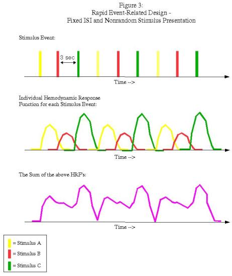
In this example, each condition follows the other in a fixed pattern: A followed by B followed by C. However, the resulting signal arising from the combination of HRFs (shown in purple in the bottom graph) is impossible to disentangle; we have no way of knowing, at any given time point, what amount of the signal is due to condition A, B, or C. In order to resolve this, we must randomize the presentation of the stimuli and also the duration of the ISI's (a process known as "jittering"):

Now we have enough variability so that we can deconvolve the contribution of each condition to the overall signal, and estimate a beta weight for each condition. This is the type of experimental design that optseq deals with.


Chapter 3: Optseq

In order to use optseq, first download the software from the MGH website (or, just google "optseq" and click on the first hit that comes up). Put the shell script into a folder somewhere in your path (such as ~/abin, if you have already downloaded AFNI) so that it will execute from anywhere within the shell. After you have done this you may also want to type "rehash" at the command line in order to update the paths. Then, type "optseq2" to test whether the program executes or not (if it does, you should get the help output, which is generated when no argument are given).

Optseq needs four pieces of information: 1) The number of time points in a block of your experiment; 2) The TR; 3) A permissible range of the minimum and maximum amounts of time after presentation of a stimulus and the start of the next (aka, the post-stimulus delay, or PSD); and 4) How many conditions there are in your experiment, as well as how long they are per trial and how many trials there are per block. Optseq will then generate a series of schedules that randomize the order  of the ITI's and the stimuli in order to find the maximum design efficiency.

Using the IAPS photos example above, let us also assume that there are: 1) 160 time points in the experiment; 2) a TR of 2 seconds; 3) A post-stimulus window of 20 seconds to capture the hemodynamic response; 3) Jitters ranging from 2 to 8 seconds; and 4) The three conditions mentioned above, each last 2 seconds per trial, and with 20 instances of DisgustingPic, 15 instances of AttractivePic, and 30 instances of NeutralPic. Furthermore, let us say that we wish to keep the top three schedules generated by optseq, each prefixed by the word IAPS, and that we want to randomly generate 1000 schedules.

Lastly, let us say that we are interested in a specific contrast - for example, calculating the difference in activation between the conditions disgustingPic and attractivePic.

In order to do this, we would type the following:

optseq2 --ntp 160 --tr 2 --psdwin 0 20 2 --ev disgustingPic 2 20 --ev attractivePic 2 15 --ev neutalPic 2 30 --evc 1 -1 0 --nkeep 3 --o IAPS --tnullmin 2 --tnullmax 8 --nsearch 1000

This will generate stimuli presentation schedules and only keep the top three; examples of these schedules, as well as an overview of how the efficiencies are calculated, can be seen in the video.


Chapter 4: The Reckoning - Comparison of optseq to 1d_tool.py

Optseq is a great tool for generating templates for stimuli presentation. However, if only one schedule is generated and applied to all blocks and all subjects, there is the potential for ordering effects to be confounded with your design, however minimal that possibility may be. If optseq is used, I recommend that a unique schedule be generated for each block, and then counterbalance or randomize those blocks across subjects. Furthermore, you may also want to consider randomly sampling the stimuli and ITI's and simulate several runs of your experiment, and then run them through AFNI's 1d_tool.py in order to see how efficient they are. With a working knowledge of optseq and 1d_tool.py, in addition to a steady diet of HotPockets slathered with Nutella, you shall soon become invincible.

You shall be...Perfect.

Unix for Neuroimagers: For Loops and Shell Scripting

With this tutorial we begin to enter into AFNI territory, as the more advanced Unix commands and procedures are necessary for running an AFNI analysis. First, we cover the basics of for loops. For loops in fMRI analysis are used to loop over subjects and execute preprocessing and postprocessing scripts for each subject individually. (By the way, I've heard of preprocessing and I've heard of postprocessing; but where does plain, regular processing take place? Has anyone ever thought of that? Does it ever happen at all? I feel like I'm taking crazy pills here.)

Within the t-shell (and I use the t-shell here because it is the default shell used by AFNI), a for loop has the following syntax:


foreach [variableName] ( [var1] [var2]...[varN])
     
     [Executable steps go here]

end


So, for example, if I wanted to loop over a list of values and have them assigned to variable "x" and then return those values, I could do something like the following:

foreach x (1 2 3 4 5)
    
     echo $x

end

Which would return the following:

1
2
3
4
5

Notice in this example that the for loop executes the line of code "echo $x", and assigns a new value to x for each step of the for loop. You can imagine how useful this can be when extended to processing individual subjects for an analysis, e.g.:

foreach subj ( subj1 subj2 subj3...subjN )

    tcsh afni_proc.py $subj

end


That is all you need to process a list of subjects automatically, and, after a little practice, for loops are easy and efficient to use. The same logic of for loops applies to FSL analyses as well, if you were to apply a feat or gfeat command to a list of feat directories. In the next batch of tutorials, we will begin covering the basics of AFNI, and eventually see how a typical AFNI script incorporates the use of for loops in its analysis.

The second part of the tutorial covers shell scripting. A shell script executes a series of commands within a text file (or, more formally, shell script), allowing the user more flexibility in applying a complex series of commands that would be unwieldy to type out in the command line. Just think of it as dumping everything you would have typed out explicitly into the command line, into a tidy little text file that can be altered as needed and executed repeatedly.

Let us say that we wish to execute the code in the previous example, and update it as more subjects are acquired. All that would be added would be a shebang, in order to specify the shell syntax used in the script:

#!/bin/tcsh

foreach subj (subj1 subj2 subj3)

     tcsh afni_proc.py $subj

end


After this file has been saved, make sure that it has executable permissions. Let's assume that the name of our shell script is AFNI_procScript.sh; in order to give it executable permissions, simply type

chmod +x AFNI_procScript.sh

And it should be able to be run from the command line. In order to run it, type the "./" before the name of the script, in order to signify that it should be executed from the shell, e.g.:

./AFNI_procScript.sh

Alternatively, if you wish to override the shebang, you can type the name of the shell you wish to execute the script. So, for example, if I wanted to use bash syntax, I could type:

bash AFNI_procScript.sh

However, since the for loop is written in t-shell syntax, this would return an error.


Due to popular demand, an optseq tutorial will be uploaded tomorrow. Comparisons between the output of optseq and AFNI's 1d_tool.py is encouraged, as there is no "right" sequence of stimulus presentations you should use; only reasonable ones.