Smoothing in AFNI

What Smoothing Is


Smoothing, the process of introducing spatial correlation into your data by averaging across nearby data points (in fMRI datasets, nearby voxels) is an essential step in any preprocessing stream. Traditionally, smoothing applies a Gaussian filter to average signal over nearby voxels in order to summate any signal that is present, while attenuating and cancelling out noise. This step also has the advantage of spreading signal over brain areas that have some variation across subjects, leading to increased signal-to-noise ratio over larger cortical areas at the loss of some spatial specificity. Lastly, smoothing mitigates the fiendish multiple comparisons problem, since voxels are not truly independent in the first place (neither are timepoints, but more on this at a later time).

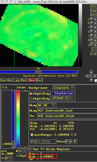
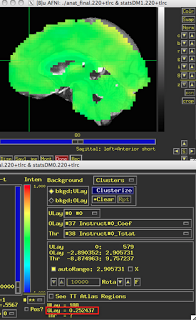
Before (left) and after (right) smoothing. Note that there is much more spatial detail in the image before smoothing is applied.


Usually this smoothing step is taken care of by your fMRI software analysis package's built-in smoothing program, but something I learned back at the AFNI bootcamp is that images coming off the scanner are already smoothed, i.e., there is already some inherent spatial correlation in the data. This makes sense, given that functional imaging datasets are acquired at relatively low resolution, and that voxels with a given intensity will most likely be immediately surrounded by other voxels with similar intensities. In the above image on the left which has not been smoothed, voxels that are brighter tend to cluster together, while voxels that are darker tend to cluster together. This spatial correlation will be increased with any additional step requiring spatial interpolation, including coregistration (aligning all volumes in a run to a reference volume), normalization (warping an image to a template space), and smoothing.


Smoothing Programs in AFNI: 3dmerge and 3dBlurToFWHM


In the good old days, the staple program for blurring in AFNI was 3dmerge with the -blur option. Since 2006, there has been a new program, 3dBlurToFWHM, which estimates the smoothness of the dataset, and attempts to smooth only to specified blur amounts in the x, y, and z directions. (Another thing I didn't recognize, in my callow youth, was that there can indeed be different smoothness amounts along the axes of your dataset, which in turn should be accounted for by your smoothing algorithm.) 3dmerge will add on the specified smoothness to whatever smoothness is already present in the data, so the actual smoothness of the data is not what is specified on the command line with 3dmerge. For example, if 3dmerge with a 6mm Full-Width at Half-Maximum (FWHM) is applied to a dataset that already has smoothness of about 3mm in the x, y, and z directions, the resulting smoothness will be about 8-9mm. (This example, similar to many simulations carried out in the lab, is not a purely linear addition, but is relatively close.)


3dBlurToFWHM, on the other hand, will begin with estimating the smoothness of your dataset, and then iteratively blur (i.e., smooth) the data until it reaches the desired level of smoothness in the x, y, and z directions. These can be specified separately, but often it is more useful to use the same value for all three. For example, the following command will blur a dataset until it reaches approximately 6mm of smoothness in each direction:

3dBlurToFWHM -FWHM 6 -automask -prefix outputDataset -input inputDataset

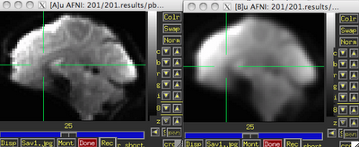
Applying this to a dataset that has been coregistered and normalized will produce output that looks like this:


Note that the first set of numbers highlighted in red are the estimates produced by 3dBlurToFWHM, and the last set of numbers of red are estimates from a separate program, 3dFWHMx. The reason for the discrepancy is that 3dBlurToFWHM uses a slightly faster and less accurate estimator when blurring; however, the two sets of numbers are functionally equivalent. In any case, the resulting blur estimates are very close to the specified FWHM kernel, typically within 10% or less.


What Mask to Use?

Often using a mask generated after the coregistration step (i.e., the 3dvolreg command) is sufficient, such as full_mask+tlrc or mask_epi_extents+tlrc. The -automask option can also be used, which usually works just as well. The only considerations to take into account are that masking out non-brain voxels will limit your field of view; some experienced users advise not masking until after performing statistical tests, as artifacts or consistent signal outside of the brain can point to hardware problems or issues with your experimental design.

What to Use for the -blurmaster Option?

According to the AFNI help for 3dBlurToFWHM, the -blurmaster option can be used to control the smoothing process, which can lead to slightly better smoothing results. As the FWHM is supposed to represent the underlying spatial structure of the noise, and not the spatial structure of the brain's anatomy, using a dataset of residuals is often a good choice here; for example, the output of -errts in 3dDeconvolve. However, this requires running 3dDeconvolve first, and then using the errts dataset in the blurmaster option all over again. This is usually more trouble than it's worth, as I haven't found significant differences between having a blurmaster dataset and not having one.


Estimating Smoothness with 3dFWHMx

After blurring your data, 3dFWHMx can be used to estimate the smoothness of a given dataset. Useful options are -geom, to estimate the geometric mean of the smoothness, and -detrend, which accounts for outlier voxels. For example,

3dFWHMx -geom -detrend -input inputDataset

What about this 3dBlurInMask Thing?

3dBlurInMask does much the same thing as 3dBlurToFWHM, except that you can use multiple masks if you desire. This procedure may also be useful if you plan to only blur within, say, the gray matter of a dataset, although this can also lead to problems such as biasing signal in certain locations after the grey matter masks have all been warped to a template space, as there is far greater variability in smoothing across masks than there is applying a smoothing kernel to the same averaged mask that incorporates all of the brain voxels across all subjects.

How to Estimate Smoothness in SPM

SPM comes with it's own smoothness estimation program, spm_est_smoothness. It requires a residuals dataset and a mask for which voxels to analyze. For example,

[fwhm, res] = spm_est_smoothness('ResMS.hdr', 'mask.hdr')

Will return the estimated FWHM in the x, y, and z directions, as well as a structure containing information about the resels of the dataset.

Why it Matters

I tuned into this problem a couple months ago when one of my colleagues got nailed by a reviewer for potentially not estimating the smoothness in his dataset appropriately. Evidently, he had used the smoothing kernel specified in his preprocessing stream when calculating cluster correction thresholds, when in fact the actual smoothness of the data was higher than that. It turned out to be a non-significant difference, and his results held in either case. However, to be on the safe side, it always helps to report estimating your smoothness with an appropriate tool. If your results do significantly change as a result of your smoothness estimation approach, then your result may not have been as robust to begin with, and may require some more tweaking.

(By tweaking, of course, I mean screwing around with your data until you get the result that you want.)

Design Efficiency: Part 2 (SPM)

As an addendum to the previous post detailing looking at regressor correlations in AFNI, a similar procedure can be done in SPM. After specifying a first-level, an SPM.mat design matrix should be generated. Navigate to the directory containing the SPM.mat file, and type "load SPM.mat".

The contents of the SPM.mat file can then be listed by just typing SPM (all caps). Running the following command will produce a NxN matrix (with N = number of regressors):

corr(SPM.xX.X)


Matching up each column to each regressor can be found in the output of SPM.xX.name

Design Efficiency

An important consideration for any fMRI experimental design is how efficiently the BOLD response will be estimated, given the timing of events and jittering between trials of interest. Therefore, before doing any scanning, it is useful to do a dry run of the experimental task on a computer outside of the scanner, and then feed this timing information into the software analysis package that you will use. For example, in SPM this would involve Specifying the 1st-Level through the SPM GUI, but not estimating it.

In AFNI, this would involve using 3dDeconvolve with the -nodata command, telling AFNI that there is no functional data to read.

#!/bin/tcsh

3dDeconvolve -nodata 205 3                       \
    -num_stimts 18                                                         \
    -stim_times 1 stimuli/reg1.txt 'GAM'                               \
    -stim_label 1 reg1                                                 \
    -stim_times 2 stimuli/reg2.txt 'GAM'                          \
    -stim_label 2 reg2                                            \
    -stim_times 3 stimuli/reg3.txt 'GAM'                     \
    -stim_label 3 reg3                                       \
    -stim_times 4 stimuli/reg4.txt 'GAM'                          \
    -stim_label 4 reg4                                            \
    -stim_times 5 stimuli/reg5.txt 'GAM'                     \
    -stim_label 5 reg5                                       \
    -stim_times 6 stimuli/reg6.txt 'GAM'                           \
    -stim_label 6 reg6                                            \
    -stim_times 7 stimuli/reg7.txt 'GAM'                      \
    -stim_label 7 reg7                                       \
    -stim_times 8 stimuli/reg8.txt 'GAM'                          \
    -stim_label 8 reg8                                            \
    -stim_times 9 stimuli/reg9.txt 'GAM'                     \
    -stim_label 9 reg9                                       \
    -stim_times 10 stimuli/reg10.txt 'GAM'                            \
    -stim_label 10 reg10                                              \
    -stim_times 11 stimuli/reg11.txt 'GAM'                       \
    -stim_label 11 reg11                                         \
    -stim_times 12 stimuli/reg12.txt 'GAM'                                  \
    -stim_label 12 reg12                                                    \
    -stim_times 13 stimuli/reg13.txt 'GAM'                              \
    -stim_label 13 reg13                                               \
    -stim_times 14 stimuli/reg14.txt 'GAM'                       \
    -stim_label 14 reg14                                         \
    -stim_times 15 stimuli/reg15.txt 'GAM'                       \
    -stim_label 15 reg15                                        \
    -stim_times 16 stimuli/reg16.txt 'GAM'                       \
    -stim_label 16 reg16                                         \
    -stim_times 17 stimuli/reg17.txt 'GAM'                           \
    -stim_label 17 reg17                                             \
    -stim_times 18 stimuli/reg18.txt 'GAM'                    \
    -stim_label 18 reg18                                      \
    -x1D X.xmat.1D -xjpeg X.jpg                                \
    -x1D_uncensored X.nocensor.xmat.1D                                     \


(A couple notes about the above code: 3dDeconvolve -nodata should be followed by the number of time points, and the TR used. In this example, I had 205 TRs, with a TR of 3 seconds, for a total of 615 seconds per run. Also, the names of the regressors have been changed to generic labels.)

The output of this command will produce estimates of how efficiently 3dDeconvolve is able to fit a model to the data provided. The Signal+Baseline matrix condition is especially important, as any singularities in this matrix (e.g., perfect or very high correlations between regressors) will make any solution impossible, as this implies that there are potentially infinite answers to estimating the beta weights for each condition. You should see either GOOD or VERY GOOD for each matrix condition; anything less than that will require using the -GOFORIT command, which can override matrix warnings. However, this should be done with caution, and only if you know what you are doing. Which I don't, most of the time.

Also notice that a number labeled the "norm. std. dev." is calculated, which is the root mean square of the measurement error variance for each condition (not to be confused with plain variance). Higher unexplained variance is less desirable, and apparently this design results in very high unexplained variance. More details about how to mitigate this, as well as a more thorough discussion of measurement error variance in general, can be found in this AFNI tutorial.


This command also produces an X.xmat.1D file, which can then be used to either visualize the regressors via 1dplot, or to examine correlations between regressors. This is done with 1d_tool.py, which is the default in the uber_subject.py stream. 1d_tool.py will set the cutoff at 0.4 before it produces any warnings, although this can be changed with the -cormat_cutoff option.

In this example, I compared two designs, one using an exponential distribution of jitters (with more jitters at shorter durations), and another which sampled equally from jitters of different durations.While the default for 1d_tool.py is to show only correlations between regressors at 0.4 or above, this can be changed using the -cormat_cutoff command, as shown below:

1d_tool.py -cormat_cutoff 0.1 -show_cormat_warnings -infile X.xmat.1D

This command produced the following output for each design:

Equal Jitters

Exponential Jitters

Note that while both do not have correlations above 0.4, there are substantial differences when looking at the range of correlations between 0.1 and 0.3. In both cases, however, each design does a relatively good job of reducing correlations between the regressors. This should also be compared against the measurement error variance as described above, as a design may produce higher correlations, but lower measurement error variance.

Final note: There are programs to create efficient designs, such as Doug Greve's optseq and AFNI's RSFgen. However, this will produce designs that are expected to be used for each subject, which potentially could lead to ordering effects. Although the likelihood of this having any significant effect on your results is small, it is still possible. In any case, all of these things should be considered together when designing a scanning study, as it takes far less time to go through these steps than to end up with an inefficient design.

Duration Modulation in AFNI

Modulating signal by duration - usually reaction time (RT) - is increasingly common in fMRI data analysis, particularly in light of recent studies examining how partialing out RT can reduce or even eliminate effects in certain regions of the brain (e.g., anterior cingulate; see Grinband et al, 2010; Yarkoni et al, 2009). In light of these findings, it appears as though parametrically modulating regressors by RT, or the duration of a given condition, is an important factor in any analysis where this data is available.

When performing this type of analysis, therefore, it is important to know how your analysis software processes duration modulation data. With AFNI, the default behavior of their duration modulation basis function (dmBLOCK) used to scale everything to 1, no matter how long the trial lasted. This may be useful for comparison to other conditions which have also been scaled the same way, but is not an appropriate assumption for conditions lasting only a couple of seconds or less. The BOLD response tends to saturate over time when exposed to the same stimulation for an extended period (e.g., block designs repeatedly presenting visual or auditory stimulation), and so it is reasonable to assume that trials lasting only a few hundred milliseconds will have less of a ramping up effect in the BOLD response than trials lasting for several seconds.

The following simulations were generated with AFNI's 3dDeconvolve using a variation of the following command:

3dDeconvolve -nodata 350 1 -polort -1 -num_stimts 1 -stim_times_AM1 q.1D 'dmBLOCK' -x1D stdout: | 1dplot -stdin -thick -thick

Where the file "q.1D" contains the following:

10:1 40:2 70:3 100:4 130:5 160:6 190:7 220:8 250:9 280:30

In AFNI syntax, this means that event 1 started 10 seconds into the experiment, with a duration of 1 second; event 2 started 40 seconds into the experiment with a duration of 2 seconds, and so on.

The 3dDeconvolve command above is a good way to generate simulation data, through the "-nodata" option which tells 3dDeconvolve that there is no functional data to process. The command tells 3dDeconvolve to use dmBLOCK as a basis function, convolving each event with a boxcar function the length of the specified duration.

Running this command as is generates the following graph:

As is expected, trials that are shorter are scaled less, while trials lasting longer are scaled more, with a saturation effect occurring around 8-9 seconds.

Running 3dDeconvolve with a basis function scaling the signal change in each to 1 is done with the following:

3dDeconvolve -nodata 350 1 -polort -1 -num_stimts 1 -stim_times_AM1 q.1D 'dmBLOCK(1)' -x1D stdout: | 1dplot -stdin -thick -thick

And generates the following output:


Likewise, the ceiling on the basis function can be set to any arbitrary number, e.g.:

3dDeconvolve -nodata 350 1 -polort -1 -num_stimts 1 -stim_times_AM1 q.1D 'dmBLOCK(10)' -x1D stdout: | 1dplot -stdin -thick -thick


However, the default behavior of AFNI is to scale events differently based on different duration (and functions identically to the basis function dmBLOCK(0)). This type of "tophat" function makes sense, because unlimited signal increase as duration also increases would lead to more and more bloodflow to the brain, which, taken to its logical conclusion, would mean that if you showed someone flashing checkerboards for half an hour straight their head would explode.

As always, it is important to look at your data to see how well your model fits the timecourse of activity in certain areas. While it is reasonable to think that dmBLOCK(0) is the most appropriate basis function to use for duration-related trials, this may not always be the case.

These last two figures show the same subject analyzed with both dmBLOCK(0) and dmBLOCK(1). The underlying beta values for each do not differ significantly, although there is some variability in how much they differ in distinct cortical areas, and small but consistent changes in variability can lead to relatively large effects at the second level.

The image on the left hasn't been masked, but the underlying beta estimates should be the same in either case.

dmBLOCK(0)
dmBLOCK(1)

Karl Friston's Rules for Reviewing

This post was orphaned a while back when I was testing links to papers, but I figured I should go back and explain what I was doing. This is a link to Friston's recent Neuroimage paper giving advice to young reviewers for how to reject any paper, regardless of how scientifically and statistically sound it is. His tone is purposely ironic, although he takes a more serious turn at the end in explaining why these rejection criteria are ridiculous.

The link to Friston's paper can be found here.

SUMA Demo

I've posted a demo of AFNI's surface mapper program, SUMA, over here on my screencast account. Specifically, I talk about how to map volumetric results generated in any fMRI software package (e.g., AFNI, FSL, SPM, BrainVoyager) onto a template surface provided by SUMA.

In this demo, I take second-level results generated in SPM and map them onto a template MNI surface, the N27 brain. All that is needed for doing this is a results dataset, a template underlay anatomical brain to visualize results on (here I use the MNI_caez_N27 brain provided in the AFNI binaries directory under ~/abin), and a folder called suma_mni that contains the .spec files for mapping onto the N27 brain. The suma_mni folder is available for download at Ziad Saad's website here. Just download it to the same directory, and you are good to go.

SPM 2nd-level results mapped onto template surface using AFNI / SUMA

I've outlined the steps in a word document, Volumetric_SUMA.docx, which is available at my website. Please send me any feedback if any of the steps are unclear.

Although this is an incredibly easy way to make great-looking figures, at the same time I would not recommend doing any ROI stats on the results mapped onto a surface using these steps. This is because it is essentially a rough interpolation of which voxel corresponds to which node; if you want to do surface ROI analyses, do all of your preprocessing and statistics on the surface (I may write up a demo of how to do this soon).

Python SUITE: AFNI_Tools.gz

This is an update from my earlier post about the Python program convertDICOM2AFNI.py; now it is a folder containing a few programs that interact with each other. The rationale was to give the original dicom conversion script a wrapper that can change directory (since I am currently unable to do this from the python interpreter invoked by the Unix shell). All the user needs to do is download the file AFNI_Tools.gz into their home directory, unzip it using "tar -zxvf AFNI_Tools.gz" into your experimental directory, and run it using the command "tcsh convertRaw2AFNI.sh". The user will be prompted for a list of subject IDs, the name of the experimental directory, and will then run the script convertDICOM2AFNI.py inside the raw fMRI data folder for each subject. This in turn will prompt the user for study-specific info, such as number of slices, number of TRs, and so on. Currently, there is no way to account for runs with different numbers of TRs; I may add this function in the future.

A short screencast demo of the suite is available at www.screencast.com/users/Andrew.Jahn/folders/Jahn_Tools (you may need to go full-screen mode in order to see what I'm typing on the command line). What I did not mention in the demo is the subfolder "Paths" within the AFNI_Tools folder. It contains two text files, groupDir.txt and dataDir.txt. groupDir.txt contains the path to the experimental directory, while dataDir.txt contains the path to the output directory that you want for each subject; these should be modified when you download the suite. I've included some documentation that I hope is enough to get people started.

In addition, after converting the raw scanner files to both AFNI and NIFTI format, the program will drive AFNI directly from the command line and allow the user to interactively scroll through each functional dataset. For example, the first run of functional data will be displayed and a video of its timecourse will start playing; this is a good way to visually check for any scanner artifacts or excessive head motion, and deciding what to do with it. You can then hit enter in the terminal window that generated AFNI, and it will skip to the next functional run of data, and so on. The idea is to make it easy to do a first-pass analysis on your raw data and see whether anything is completely out of line.

As always, please send me feedback if you have actually used the program, and what you think about it.


=====================
P.S. Photos from the AFNI bootcamp are now up. I now have photographic evidence that I was at the National Institutes of Health, and not somewhere else, like Aruba.

AFNI Bootcamp / Proof that I was not in Aruba

Ye Good Olde Days

I've uploaded my powerpoint presentation about what I learned at the AFNI bootcamp; for the slides titled "AFNI Demo", "SUMA Demo", and so on, you will have to use your imagination.

The point of the presentation is that staying close to your data - analyzing it, looking at it, and making decision about what to do with it - are what we are trained to do as cognitive neuroscientists (really, any scientific discipline). The reason I find AFNI to be superior is that it allows the user to do this in a relatively easy way. The only roadblocks are getting acquainted with Unix and shell programming, and also taking the time to get a feel for what looks normal, and what looks potentially troublesome.


Back in the good old days (ca. 2007-2008) we would simply make our scripts from scratch, looking through fMRI textbooks and making judgments about what processing step should go where, and then looking up the relevant commands and options to make that step work. Something would inevitably break, and if you were like me you would spend days or weeks trying to fix it. To make matters worse, if you asked for help from an outside source (such as the message boards), nobody had any idea what you were doing.

The recent scripts containing the "uber" prefix - such as "uber_subject.py", "uber_ttest.py", and so on - have mitigated this problem considerably, generating streamlined scripts that are more or less uniform across users, and therefore easier to compare and troubleshoot. Of course, you still need to go into the generated script and make some modifications here and there, but everything is pretty much in place. It will still suggest that you check each intermediate step, but that becomes easier to ignore once you have a higher-level interface that takes care of all the minor details for you. Like everything else, there are tradeoffs.

Python Script: convertDICOM2AFNI.py

I've written my first (useful) python script, a small program called convertDICOM2AFNI.py, that looks for DICOM files from our scanner and converts them to AFNI format. Converting raw scanner data to AFNI format using the to3d command is light years (i.e., minutes) faster than SPM's DICOM import, or MRIcron's dcm2nii program. dcm2nii, in particular, usually gave me a bunch of other files that I was never interested in and would convert everything in my raw DICOM folder, even though there were only a few runs that I was interested in looking at. It would also introduce some weird temporal interpolations into the data, modifying the header information to make it appear as though the volumes were slice-time corrected even though they actually were not.

In order to get around this problem, I may add an option to the script which converts to AFNI, and then converts to nifti format using 3dAFNI2NIFTI (although I have no idea what might get lost in the translation; will need to do some testing here).

To use the script, do the following:

1) Create folder containing all raw DICOM files generated from your experiment
2) Write down which session numbers correspond with which functional and anatomical runs (remember: pencil & paper are your friends)
3) Run the script from the raw DICOM directory using the command "python convertDICOM2AFNI.py"

It will ask you a series of questions about which session numbers are your functional runs, and then which session is your anatomical run. If you run the command without defaults (i.e., without using the "-d") flag, it will also ask you the number of slices in the z-direction, the number of TRs, and the length of each TR in milliseconds.

In the future, I plan to have the program automatically read in a defaults file that specifies all of these arguments automatically. However, that also assumes that the user is organized (which I am not). Also, as of this writing, it assumes that the z-slices alternate positively in the z-direction; if this is not true for you, you may need to change the script yourself.

The script is available for download over at my webpage (http://mypage.iu.edu/~ajahn) under "Python Scripts". The actual location of the scripts I write will probably change as I become more organized.


I plan to begin writing a suite of Python programs that I find useful for interacting with both SPM and AFNI data, eventually working up to a GUI sometime in the far future. For now, it will assume a degree of command line proficiency and that you can probably figure things out if the script does not perfectly fit your needs.


===============================

Due to high demand from the Scottish population at IU, a screencast will soon be up detailing how to interpolate volumetric data onto a template surface.